Reformulating a Problem

As explained in the Getting Started with D-Wave Solvers guide, the first step of solving your problem is to state it; for example:

• How do I assign a color to each region of a map such that any two regions sharing a border have different colors? (This is the well-known Map Coloring problem.)

• How do I find values of the binary variables that satisfy the satisfiability (SAT) problem,

  \[(x_1 \vee \overline{x}_2 ) \wedge (\overline{x}_1 \vee x_2)\]

• How do I place routers in a communications network for maximum coverage of all network nodes? (This can be posed as the vertex cover problem as done in the vertex cover example.)

The next step is to map the problem to an objective function, usually in Ising or QUBO formats[1] if you are submitting to a quantum sampler, known as the quantum computer’s native formulations. Low-energy states of the objective function represent good solutions to the problem.

[1]

These belong to the category of binary quadratic models (BQM). Leap‘s quantum-classical hybrid solvers can accept problems formulated at a higher level of abstraction; for example, discrete quadratic models (DQM), where variables can have more than two possible cases.

This chapter presents some general guidance, the following reformulation techniques[2], and some extended reformulation examples:

[2]

Some of these techniques are intended for use with quantum samplers and Leap’s hybrid solvers that accept binary quadratic models; for example, if you are using a constrained quadratic model (CQM) solver, you can state constraints in a straightforward manner.

The sections also provide references to examples and literature to guide understanding and implementation.

Note

Some sections describe the techniques in formal mathematical formulation, which might be abstract, but those typically also provide simple examples for users looking for practical guidance.

General Guidance on Reformulating

While Leap‘s hybrid solvers can accept arbitrarily structured BQMs of huge size, problems submitted directly to the quantum computer must be formulated to be compatible with the constraints of the physical system and as robust as possible to its control errors[3].

[3]

The QPU Solver Datasheet guide provides details on the physical system and its integrated control errors (ICE).

Reformulation Steps

To map a problem to a quadratic model, you can try the following steps.

1. Write out the objective and constraints.

   This should be written out in terms of your problem domain, not necessarily in math format.

   • The objective of a problem is what you are looking to minimize[4].

   • A constraint in a problem is a rule that you must follow; an answer that does not satisfy a given constraint is called infeasible, it’s not a good answer, and might not be usable at all. For example, a travelling salesperson cannot be in two cities at once or the trucks in your problem may not be able to hold more than 100 widgets.

   There may be more than one way to interpret your problem in terms of objectives and constraints.

2. Convert objective and constraints into math expressions.

   Decide on the type of variables to best formulate it:

   • Binary

     Does your application optimize over decisions that could either be true (or yes) or false (no)? For example,

     • Should the antenna transmit or no?

     • Did a network node experience failure?

   • Discrete

     Does your application optimize over several distinct options? For example,

     • Which shift should employee X work?

     • Should the state be colored red, blue, green or yellow?

   • Integer

     Does your application optimize the number of something? For example,

     • How many widgets should be loaded onto the truck?

   • Continuous

     Does your application optimize over an uncountable set? For example,

     • Where should the sensor be built?

   Once you think of a problem in these terms, you can assign a variable for each question.

   Next ask about the degree the problem can likely be formulated as:

   • Quadratic

     Are its relationships defined pairwise? For example,

     • In the structural imbalance example each pair of people in the network is either friendly or hostile.

   • Higher-Order

     Does your application have relationships between multiple variables at once? For example,

     • Simulating an AND gate

   Next, transform objective and constraints into math expressions. For binary variables, this can often be done with truth tables if you can break the problem down into two- or three-variable relationships. For other variables and non-quadratic degrees, you can try techniques such as Non-Quadratic (Higher-Degree) Polynomials and Ocean tools such as Higher-Order Models.

3. Reformulate as a quadratic model.

   Different types of expressions require different strategies. Expressions derived from truth tables may not need any adjustments. The D-Wave Problem-Solving Handbook provides a variety of reformulation techniques; some common reformulations are:

   • Squared terms: QUBO and Ising models do not have squared binary variables. In QUBO format, its 0 and 1 values remain unchanged when squared, so you can replace any term \(x_i^2\) with \(x_i\). In Ising format, its -1 and +1 values always equal 1 when squared, so you can replace any term \(s_i^2\) with the constant 1.

   • Maximization to minimization: if your objective function is a maximization function (for example, maximizing profit), you can convert this to a minimization by multiplying the entire expression by -1. For example:

     \[\mbox{arg max} (3v_1+2v_1v_2) = \mbox{arg min} (-3v_1-2v_1v_2)\]

   • Equality to minimization: if you have a constraint that is an equality, you can convert it to a minimization expression by moving all arguments and constants to one side of the equality and squaring the non-zero side of the equation. This leaves an expression that is satisfied at its smallest value (0) and unsatisfied at any larger value (>0). For example, the equation \(x+1=2\) can be converted to \(\min_x[2-(x+1)]^2\), which has a minimum value of zero for the solution of the equation, \(x=1\).

     This approach is useful also for \(n \choose k\) constraints (selection of exactly \(k\) of \(n\) variables), where you disfavor selections of greater or fewer than \(k\) variables with the penalty \(P = \alpha (\sum_{i=1}^n x_i - k)^2\), where \(\alpha\) is a weighting coefficient (see penalty method) used to set the penalty’s strength.

4. Combine expressions.[5]

   Once you have written all of the components (objective and constraints) as quadratic models, for example BQMs, make a final BQM by adding all of the components. Typically you multiply each expression by a constant that weights the different constraints against each other to best reflect the requirements of your problem. You may need to tune these multipliers through experimentation to achieve good results. You can see examples in Ocean software’s collection of code examples on GitHub.

[4]

For maximization see step 3.

[5]

When using penalty models for constraints.

Reformulation Considerations

You can frequently reformulate a problem in a variety of ways, some of which may be more performant than others. This section notes some general considerations and common practices for successful reformulation.

Compare Approaches

Start with the simplest possible method you can find to formulate your problem in the supported format of your chosen solver (BQM, CQM, etc). If your formulation does not provide good solutions (with the solver properly configured), consider alternative formulations. A formulation that has the disadvantage of increasing the number of variables might compensate by being more amenable to minor-embedding; a different formulation might produce a smaller range of bias values.

Variable Proliferation

Some reformulations may create very large numbers of variables; for example, integer-to-binary-variables conversion typically does. There may be alternative formulations that require fewer variables.

For example, although you may be able to derive a penalty by conversion to a linear equality or by conversion to a linear inequality, it may produce better solutions to apply the techniques of the non-linear constraints section to construct a penalty with fewer ancillary variables. [6]

[6]

Equality constraints, \(\sum_{i=0}^N a_ix_i == b\), standardly formulated as BQMs,

\[\text{E}(\vc x) = \left( \sum_{i=0}^N a_ix_i - b \right)^2\]

require about \(N^2/2\) biases. For 20 such constraints, you need about 200 biases; for 2000 constraints you already need about two million biases.

For a particular example, consider the constraint \(x_1\vee x_2\vee x_3\) (which is useful for solving a 3-SAT). You can express it as the inequality \(x_1+x_2+x_3\ge 1\) and convert it to the penalty function

\[(x_1+x_2+x_3 - 1 -a_1-2a_2)^2.\]

The two ancillary variables \(a_1\) and \(a_2\) are necessary to represent the possible slack values 0, 1, and 2. However, the penalty function

\[-3+ (\overline{x}_1+\overline{x}_2+\overline{x}_3)(1+a) + \overline{a} + x_1 x_2 + x_2 x_3 + x_3 x_1\]

represents the same constraint using a single ancillary variable.[7]

[7]

In fact, this representation is commonly used to reduce 3-SAT to MAX-2-SAT.

Section Energy Gap shows a small example of two formulations of the same penalty function with different numbers of ancillary variables.

Scale of Biases

The scale of biases—the difference between the smallest and largest biases in your BQM—can affect performance. For QPU solvers, your BQM’s linear and quadratic coefficients translate in the end to qubit and coupler biases; if your problem results in, for example, a smallest bias of \(h_{12}=-0.032\) and a largest bias of \(h_{36}=3405\), when these biases are scaled down to the range of biases supported on the QPU, h_range, the small bias is effectively zero.

Pay attention to the scale of biases in your selected formulation—sometimes small formulation changes can produce much lower scales.

Section Problem Scale shows a code example.

Clearer Representations

Some formulations might be more intuitive than others, and therefore easier to use and debug. For example, you can lower-bound a QUBO by rewriting without any negative coefficients, using negative literals instead: express contributions such as \(-3 x_1 x_2\) as either

\[-3+3\overline{x}_2+3\overline{x}_1 x_2 \qquad \text{or} \qquad -3+3\overline{x}_1+3x_1\overline{x}_2.\]

The alternative expressions clearly show a lower bound of \(-3\).

Similarly, some formulations allow you to make the value of the energy meaningful. This can be useful in understanding the quality of solutions.

Further Information

• [dwave1] provides step-by-step guidance and exercises for modeling small problems using BQMs.

• [Kar2017] presents an approach for encoding integer variables into binary ones for use in representing unconstrained integer quadratic programming problems in QUBO format.

Algorithms Implemented in Ocean

Some problem categories are common enough that you can find existing implementations of the reformulation.

Example: Graph Problems

Ocean software provides algorithms for many known graph problems.

This example demonstrates a problem of finding the largest group of friends who all know each other in a social setting. It states the problem as the graph problem maximum clique. Instead of working out the mathematical mapping to a BQM yourself, you can use Ocean’s dwave_networkx.clique_number() function.

>>> import networkx as nx
>>> import dwave_networkx as dnx
>>> import dimod
>>> # Create an illustration graph
>>> G = nx.caveman_graph(2, 4)
>>> dnx.algorithms.clique.clique_number(G, dimod.ExactSolver())
4

Example: Constraints

Ocean software provides generic quadratic-model generators.

This example shows how you can use a dimod BQM generator for a problem that includes a constraint \(n \choose k\), which requires that exactly \(k\) of \(n\) variables be selected. The dimod.generators.combinations() function builds a BQM that is minimized when exactly \(k\) of its variables equal 1.

>>> import dimod
>>> bqm_4_2 = dimod.generators.combinations(['x1', 'x2', 'x3', 'x4'], 2)

Adding the bqm_4_2 BQM to a problem BQM with variables x1, x2, x3, x4, with a suitable weight (see penalty method) makes it probable that exactly two of the four variables are 1 in returned solutions.

>>> print(dimod.ExactSolver().sample(bqm_4_2).first)     
Sample(sample={'x1': 1, 'x2': 1, 'x3': 0, 'x4': 0}, energy=0.0, num_occurrences=1)

Further Information

• See the Ocean documentation for available BQM-generating functionality.

Native QPU Formulations: Ising and QUBO

You may be able to formulate some problems directly as binary quadratic models, as shown in the examples of the Getting Started with D-Wave Solvers guide.

Reminder: Ising and QUBO formulations

The D-Wave QPU can be viewed as a heuristic that minimizes Ising objective functions using a physically realized version of quantum annealing.

In Ising formulation, given a problem of \(N\) variables corresponding to physical Ising spins, \(\vc s=[s_1,...,s_N]\), and a configuration of \(h_i\) local fields and \(J_{i,j}\) couplings between spins, the QPU (in its solution spin values) minimizes the objective function

\[\begin{split}\begin{array}{lll} E(\vc{s} | \vc{h}, \vc{J}) = & & \\ \sum_{i=1}^N h_i s_i & & \\ + \sum_{i<j}^N J_{i,j} s_i s_j & & \end{array}\end{split}\]

It is straightforward to translate between Ising and QUBO representations. In QUBO formulation, \(N\) binary variables are represented as an upper-diagonal matrix \(\vc{Q}\), where diagonal terms are the linear coefficients and the nonzero off-diagonal terms are the quadratic coefficients. The objective function to minimize is

\[ \begin{align}\begin{aligned} E(\vc{x}| \vc{Q}) &= \sum_{i\le j}^N x_i Q_{i,j} x_j\\&= \ip{\vc{x}}{\vc{Q}\vc{x}}\end{aligned}\end{align} \]

For many small problems—or large problems amenable to being broken into small parts—you can use truth tables to construct a BQM. For many others, the original mathematical formulation can simply be mapped to Ising or QUBO format. Others might enable formulation through known elements such as Boolean logic or simple penalty models.

Example: Truth-Table Formulation

As shown in the Getting Started with D-Wave Solvers guide, you can formulate a QUBO in the following steps:

1. Tabulate all the problem’s possible states in a truth table.

2. Penalize undesirable states with higher energies.

3. Set QUBO coefficients that result in the selected energies for each state.

This example uses a truth table to formulate the NOT constraint, \(v_2 = \neg v_1\). A penalty (energy gap) of 1 is chosen.

Table 11 shows all four possible states of \(v_1, v_2\) in columns two and three, whether the state is feasible for constraint \(v_2 = \neg v_1\) in column four, and a relative penalty of 1 for the infeasible states in the rightmost column.

Table 11 Truth Table to Formulate a QUBO for NOT constraint

State	\(v_1\)	\(v_2\)	\(v_2 = \overline{v_1}\) ?	Penalty
1	0	0	No	p
2	0	1	Yes	p-1
3	1	0	Yes	p-1
4	1	1	No	p

Substituting the values of the table’s variables for variables \(q_1, q_2\) in the two-variable QUBO model,

\[E(a_i, b_{i,j}; q_i) = a_1 q_1 + a_2 q_2 + b_{1,2} q_1 q_2,\]

and the desired penalty for the resulting energy produces for the four rows of the table these four equalities:

\[\begin{split}\text{State 1:} \qquad a_1 0 + a_2 0 + b_{1,2} 00 &= p \\ \text{State 2:} \qquad a_1 0 + a_2 1 + b_{1,2} 0 1 &= p-1 \\ \text{State 3:} \qquad a_1 1 + a_2 0 + b_{1,2} 1 0 &= p-1 \\ \text{State 4:} \qquad a_1 1 + a_2 1 + b_{1,2} 1 1 &= p\end{split}\]

Giving the following four equations with four variables:

\[\begin{split}0 &= p \\ a_2 &= p-1 \\ a_1 &= p-1 \\ a_1 + a_2 + b_{1,2} &= p\end{split}\]

Solving these equations by simple substitution gives \(E(q_1, q_2) = -q_1 - q_2 +2 q_1 q_2\), which is equivalent to the QUBO given in Table 17 of the Elementary Boolean Operations section, with an offset of 1 (this formulation has a ground-state energy of -1 versus the other formulation’s ground-state energy of 0).

Example: Formulation by Similarity

Problems formulated as either a maximum independent set (MIS), which seeks the largest subset of vertices of graph \(G=(V,E)\) that have no common edge, or a maximum cut, which seeks a subset of vertices that maximizes the number of edges between the subset and remaining vertices, have a noticeable similarity to the Ising format.

In MIS formulation, the objective function is:

\[\text{MIS:} \qquad \text{E}(\vc x) = - \sum_{i\in V} x_i + \sum_{(i,j)\in E} M_{i,j} x_i x_{j}.\]

Clearly this formulation is similar to Ising with local fields \(h_i=-1\) and only positive coupling strengths \(J_{i,j}\) (represented by penalties \(M_{i,j}>1\)).

You can formulate such problems as BQMs yourself but Ocean software’s dwave_networkx provides functions for these graph problems and more.

Example: Formulation with Boolean Logic

The technique of formulating problems with Boolean operations is very versatile: modern computing is built on Boolean gates, the scope of addressable problems is immense.

To express a constraint that variable \(z\) should be 1 if either or both of variables \(x1\) or \(x2\) are one, you can use an OR gate. Ocean’s dimod provides functionality for creating BQMs from Boolean logic:

>>> from dimod.generators import or_gate
>>> from dimod import ExactSolver
>>> # Create an OR constraint
>>> bqm_or = or_gate('x1', 'x2', 'z')
>>> # View best solutions
>>> print(ExactSolver().sample(bqm_or).lowest(atol=0.7))
  x1 x2  z energy num_oc.
0  0  0  0    0.0       1
1  0  1  1    0.0       1
2  1  1  1    0.0       1
3  1  0  1    0.0       1
['BINARY', 4 rows, 4 samples, 3 variables]

The lowest-energy solutions are all feasible solutions for the constraint.

The factoring example expresses the constraints of a CSP with Boolean logic. The approach used in that example is to express \(P=ab\) as a CSP with a binary multiplication circuit.

Section Elementary Boolean Operations below shows QUBO formulation for a number of common Boolean operators.

Ising or QUBO?

Some problems are better formulated as QUBOs, some as Ising models. The maximum independent set of the Example: Formulation by Similarity section clearly maps well to an Ising formulation, for example, as does the structural imbalance problem solved in structural imbalance example.

Consider both when mapping a problem and compare ease of formulation and later solution quality.

You can use the simple arithmetic mapping, \(\vc{s}=2\vc{x}-\vc{1}\), where \(\vc{1}\) is the vector all of whose components are 1, to translate between these native formulations:

\[ \ip{\vc{x}}{\vc{Q}\vc{x}} = \frac14 \ip{\vc{1}}{\vc{Q}\vc{1}} + \ip{\overbrace{\vc{Q}\vc{1}/2}^{\vc{h}}}{\vc{s}} + \ip{\vc{s}}{\overbrace{(\vc{Q}/4)}^{\vc{J}}\vc{s}}\]

Thus,

\[E(\vc{x}|\vc{Q}) = \ip{\vc{1}}{\vc{Q}\vc{1}} + E(\vc{s}|\vc{Q}\vc{1}/2, \vc{Q}/4).\]

Example

The Example Reformulation: Map Coloring section develops an objective function, in QUBO formulation,

\[\text{E}(a_i, b_{i,j}; q_i) = -q_B -q_G + 2q_B q_G,\]

where \(q_B\) is a variable representing blue and \(q_G\) green.

You can view this Ising formulation using the inverse of the \(\vc{s}=2\vc{x}-\vc{1}\) Ising-to-QUBO conversion. For this objective function, the variables are

\[\begin{split}\vc{x} = \begin{bmatrix} q_B \\ q_G \end{bmatrix} \qquad \vc{s} = \begin{bmatrix} s_B \\ s_G \end{bmatrix}\end{split}\]

The inverse conversion in scalar form, \(q_i=\frac{s_i+1}{2}\), is a simple mathematical manipulation of \(s_i=2x_i-1\), where the QUBO variables in scalar form are \(x_1,x_2=q_B,q_G\). Substituting in the objective function yields

\[ \begin{align}\begin{aligned} \text{E}(h_i, j_{i,j}; s_i) &= -\frac{s_B+1}{2} -\frac{s_G+1}{2} + 2 \frac{s_B+1}{2} \frac{s_G+1}{2}\\&= \frac{1}{2}(s_Bs_G-1).\end{aligned}\end{align} \]

Ocean software can automate such conversions for you:

>>> import dimod
>>> dimod.qubo_to_ising({('qb', 'qb'): -1, ('qg', 'qg'): -1, ('qb', 'qg'): 2})
({'qb': 0.0, 'qg': 0.0}, {('qb', 'qg'): 0.5}, -0.5)

Table 12 shows the two formulations’ identical energy functions, with minimum levels for the valid states of a single selected color, either blue (\(0,1\) in a QUBO or \(-1,1\) in an Ising model) or green (\(1,0\) or \(1,-1\)).

Table 12 Ising Equivalent of QUBO

\(\mathbf{q_B,q_G}\)	\(\mathbf{s_B,s_G}\)	\(\mathbf{\text{E}(a_i, b_{i,j}; q_i)=\text{E}(h_i, j_{i,j}; s_i)}\)
\(0,0\)	\(-1,-1\)	\(0\)
\(0,1\)	\(-1,1\)	\(-1\)
\(1,0\)	\(1,-1\)	\(-1\)
\(1,1\)	\(1,1\)	\(0\)

For example, the state \(q_B,q_G=0,1\) of the second row is represented by the QUBO penalty function,

\[ \begin{align}\begin{aligned}\text{E}(a_i, b_{i,j}; q_i) &= -q_B -q_G + 2q_B q_G,\\&= -0 - 1 +2 \times 0 \times 1\\&= -1\end{aligned}\end{align} \]

while the equivalent state \(s_B,s_G=-1,1\) of that same row is represented by the Ising penalty function,

\[ \begin{align}\begin{aligned}\text{E}(h_i, j_{i,j}; s_i) &= \frac{1}{2}(s_Bs_G-1)\\&= \frac{1}{2}(-1 \times 1 -1) = \frac{-2}{2}\\&= -1\end{aligned}\end{align} \]

with the same resulting penalty.

Note that the constant \(-\frac{1}{2}\) in the Ising formulation above, which does not affect the relative energies, does not map into the formulation used to configure the D-Wave system, and is discarded.

Further Information

• [Bar1982] shows that Ising and QUBO problems are NP-hard.

• [Ber1999] discusses a broad tractable subclass of Ising problems in the context of rounding algorithms.

• [Bru1967] provides a history of the Lenz-Ising model and its uses.

• [Cou2009] and [Sch2009] discuss particular cases of tractable Ising problems.

• [Koc2004] and related papers show that QUBOs are an effective representation for modeling and solving a variety of discrete optimization problems.

• [Kol2004] characterizes binary-variables energy functions that can be minimized by graph cuts.

• [Luc2013] and [Lod2020] describe Ising formulations of many NP problems.

Weighted MAX-2-SAT

The SAT problem problem is to decide whether the literals in its clauses can be assigned values that satisfy all the clauses; i.e., produce a value of \(1\). In CNF, the SAT is satisfied only if all its clauses are satisfied.

SAT Terminology

• Literal is a Boolean variable such as \(x_i\) and \(\overline{x_i}\).

• Clause is a disjunction of literals such as \(x_i \vee \overline{x_j}\).

• conjunctive normal form (CNF) conjoins clauses by the AND operator; i.e., (clause 1) \(\wedge\) (clause 2).

The Simple Satisfiability (SAT) Example of the Getting Started with D-Wave Solvers guide demonstrated an intuitive formulation of a small SAT as a BQM. This section provides a more methodological approach.

A 2-SAT has \(m\) clauses of 2 literals each. A MAX-2-SAT is the problem of assigning values that maximize the number of satisfied clauses (an optimization problem; a second version is to decide whether some specified number of clauses can be satisfied). Weighted MAX-SAT assigns each clause a positive weight so the violation of clause \(c\) incurs a cost \(w_c\) and the problem is to maximize the weight of satisfied clauses

\[\text{MAX-2-SAT:} \qquad \underbrace{(\ell_{c1,1} \vee \ell_{c1,2} ; w_{c1})}_{\text{clause 1}} \wedge \underbrace{(\ell_{c2,1} \vee \ell_{c2,2} ; w_{c2})}_{\text{clause 2}} \wedge ... \wedge \underbrace{(\ell_{cm,1} \vee \ell_{cm,2} ; w_{cm})}_{\text{clause m}}\]

where \(\ell_{ci,1}\) and \(\ell_{ci,2}\) are the two literals of clause \(ci\), and \(w_{ci}\) is its weight.

To reformulate a MAX-2-SAT problem as a QUBO, note that (1) maximizing the weight of satisfied clauses is equivalent to minimizing the weight of unsatisfied clauses, and (2) by De Morgan’s laws, \(\overline{x_i \vee x_j} = \overline{x_i} \wedge \overline{x_j}\).[8] This means that the general weighted MAX-2-SAT problem can be written as a posiform (in the context of machine learning problems, a polynomial expression that conjoins AND clauses with OR operations) that minimizes the weight of unsatisfied clauses:

\[\min_{\vc{x}} \sum_c w_c \overline{\ell}_{c,1} \overline{\ell}_{c,2}.\]

[8]

For an intuitive understanding, verify with a truth table that clause \(x_1 \vee \overline{x}_2\) is unsatisfied if \(\overline{x}_1 \wedge x_2\) is true, and this conjunction is equivalent to the product of Boolean variables \(\overline{x}_1 x_2\). If weighted clause \((x_1\vee \overline{x}_2; 3)\) is unsatisfied a cost of 3 is incurred, thus the penalty representing the clause is \(3 \overline{x}_1 x_2\).

Example: Converting a Three-Variable MAX-2-SAT to a QUBO

Consider the following weighted MAX-2-SAT on three variables, \(x_1,x_2,x_3\), with weights \(w_{c1}=3, w_{c2}=1, w_{c1}=4\), which maximizes the number of satisfied clauses on,

\[\underbrace{(x_1\vee \overline{x}_2; 3)}_{\text{clause 1}} \wedge \underbrace{(x_3;1)}_{\text{clause 2}} \wedge \underbrace{(\overline{x}_3 \vee x_2;4)}_{\text{clause 3}}.\]

Obtain the QUBO representation using these steps:

1. Formulate as a posiform (using \(\overline{x_i \vee x_j} = \overline{x_i} \wedge \overline{x_j}\) and minimizing the weight of unsatisfied clauses as explained above):

\[\min_{\vc{x}} \left\{ \underbrace{3(\overline{x_1} \wedge x_2)}_{\text{clause 1}} + \underbrace{1(\overline{x_3})}_{\text{clause 2}} + \underbrace{4(x_3 \wedge \overline{x_2})}_{\text{clause 3}} \right\} = \min_{\vc{x}} \left\{3\overline{x_1} x_2 +\overline{x_3}+4x_3 \overline{x_2}\right\}.\]

2. Write negated literals \(\overline{x_i}\) as \((1-x_i)\):

\[ \begin{align}\begin{aligned}\min_{\vc{x}} \left\{3(1-x_1) x_2+(1-x_3)+4x_3 (1-x_2)\right\}\\= \min_{\vc{x}} \left\{3x_2 -3x_1x_2 +1 - x_3 + 4x_3 - 4x_2x_3 \right\}\\= \min_{\vc{x}} \left\{1 + 3x_2 + 3x_3 -3x_1x_2 - 4x_2x_3 \right\}\end{aligned}\end{align} \]

In this last expression, the example weighted MAX-2-SAT has been reformulated as a QUBO in scalar notation,

\[\text{E}_{qubo}(a_i, b_{i,j}; x_i) = \sum_{i} a_i x_i + \sum_{i<j} b_{i,j} x_i x_j,\]

where \(a_1=0, a_2=3, a_3=3\) are the linear coefficients and \(b_{1,2}=-3, b_{2,3}=-4\) the quadratic coefficients.

Further Information

• [Bon2007] generalizes the resolution rule for satisfiability to weighted MAX-SAT, which enables the simplification of some weighted MAX-2-SAT problems.

• [Coo1971] and [Lev1973] identify satisfiability as the first NP-complete problem. (Finding a satisfiable assignment or proving that there is no satisfying assignment for 2-SAT can be done in polynomial time. However, 3-SAT which allows clauses of up to 3 literals is NP hard and there are problem instances which cannot be solved in polynomial time.)

• [Wat2006] discusses the average-case complexity of the MAX-2SAT problem.

Non-Quadratic (Higher-Degree) Polynomials

To reduce problems with interactions between more than pairs of variables to a QUBO, introduce and minimize over ancillary variables.

A good procedure is to select the pair of variables that is most common amongst all terms with more than pairwise interactions, and replace it with an ancillary variable in all those terms. Repeat until no more terms of 3 or more variables remain. Note that subsequent iterations may involve products of ancillary variables if these ancillary pairs are the most common amongst the terms.

An interaction involving 4 or more variables can be reduced to pairwise by sequentially introducing new variables and reducing the degree of the interaction by 1 at each step.

Below are two techniques you can use. Ocean software can automate such reduction for you:

>>> import dimod
>>> cubic = {('x',): -1, ('y',): 1, ('z',): 1.5, ('x', 'y'): -1, ('x', 'y', 'z'): -2}
>>> print(dimod.make_quadratic(cubic, 5, dimod.BINARY))        
BinaryQuadraticModel({x: -1.0, y: 1.0, z: 1.5, z*x: 15.0},
{('x', 'y'): -1, ('x', 'z'): 5.0, ('x', 'z*x'): -10.0, ('y', 'z*x'): -2,
('z', 'z*x'): -10.0}, 0.0, 'BINARY')

Polynomial Reduction by Minimum Selection

To reformulate a non-quadratic (higher-degree) polynomial to Ising/QUBO, substitute terms in the form of \(axyz\), where \(a\) is a real number, with one of the following quadratic terms:[9]

\[ \begin{align}\begin{aligned}axyz = aw ( x+y+z -2) \quad a<0\\axyz = a \left\{ w ( x+y+z -1) + (xy+yz+zx) - (x+y+z) +1 \right\} \quad a>0\end{aligned}\end{align} \]

[9]

It is easy to verify, for example, that the equality for the negative coefficient, \(a<0\), holds. The term \(( x+y+z -2)\) is positive and non-zero only for \(x,y,z=1,1,1\), so multiplying by negative \(a\) yields the only negative value of \(w ( x+y+z -2)\), which is preserved for \(w=1\). All other states of \(x,y,z\) result in \(( x+y+z -2) \le 0\), so multiplied by \(a<0\) yield zero or positive values, which are minimized to zero by \(w=0\).

This technique of reduction by minimum selection exploits the identity,

\[xyz = \max_w \left\{ w ( x+y+z -2) \right\}\]

where \(x,y,z\) are binary variables in some pseudo-binary function being minimized and \(w\) is the ancillary binary variable introduced to substitute quadratic terms for cubic terms.

Table 13 shows that the cubic and quadratic formulations are identical. In this table, column \(\mathbf{x,y,z}\) is all possible states of the \(xyz\) term and column \(\mathbf{xyz}\) is the corresponding values of the \(xyz\) term; column \(\mathbf{x+y+z-2}\) is an intermediate calculation, the right side of the equality without the ancillary variable and before maximization, shown for clarity; and column \(\mathbf{\max_w\left\{w(x+y+z-2)\right\}}\) is the final result of calculating the right side of the equality.

Table 13 Minimum Selection Reduction.

\(\mathbf{x,y,z}\)	\(\mathbf{xyz}\)	\(\mathbf{x+y+z-2}\)	\(\mathbf{\max_w\left\{w(x+y+z-2)\right\}}\)
\(0,0,0\)	\(0\)	\(-2\)	\(0|_{w=0}\)
\(0,0,1\)	\(0\)	\(-1\)	\(0|_{w=0}\)
\(0,1,0\)	\(0\)	\(-1\)	\(0|_{w=0}\)
\(0,1,1\)	\(0\)	\(0\)	\(0|_{w=0,1}\)
\(1,0,0\)	\(0\)	\(-1\)	\(0|_{w=0}\)
\(1,0,1\)	\(0\)	\(0\)	\(0|_{w=0,1}\)
\(1,1,0\)	\(0\)	\(0\)	\(0|_{w=0,1}\)
\(1,1,1\)	\(1\)	\(1\)	\(1|_{w=1}\)

Example

This simple example solves higher-order polynomial \(-x +2y +3z +xy -2xyz\) in two ways: first, using an Ocean higher-order solver; second, using a quadratic solver on the reduced form.

>>> import dimod
>>> hubo = {('x', 'x'): -1, ('y', 'y'): 2, ('z', 'z'): 3, ('x', 'y'): 1,
...         ('x', 'y', 'z'): -2}
>>> qubo = {('x', 'x'): -1, ('y', 'y'): 2, ('z', 'z'): 3, ('w', 'w'): 4,
...         ('x', 'y'): 1, ('w', 'x'): -2, ('w', 'y'): -2, ('w', 'z'): -2}
>>> print(dimod.ExactPolySolver().sample_hubo(hubo).first)
Sample(sample={'x': 1, 'y': 0, 'z': 0}, energy=-1.0, num_occurrences=1)
>>> print(dimod.ExactSolver().sample_qubo(qubo).first)
Sample(sample={'w': 0, 'x': 1, 'y': 0, 'z': 0}, energy=-1.0, num_occurrences=1)

Polynomial Reduction by Substitution

To reformulate a non-quadratic polynomial to Ising/QUBO, use this substitution to reduce a triplet interaction to pairwise,

\[x_1 x_2 x_3 = \min_z \bigl\{ z x_3 + M P(x_1,x_2;z) \bigr\},\]

where \(M>1\) is a penalty weight and \(P\) is some penalty function that has lowest value when \(z = x_1 x_2\). This reformulation is quadratic—the lefthand term, \(z x_3\), multiplies two variables, \(z\) and \(x_3\), and the righthand term, \(P(x_1,x_2;z)\) is a quadratic penalty function—and has lowest values for configurations of variables where \(z x_3 = x_1 x_2 x_3\).

Example Example: Boolean Variables shows such a reduction for binary-valued variables while Example: Spin Variables shows it for spin-valued variables.

Example: Boolean Variables

This example of reduction by substitution represents the multiplication \(x_1 x_2\) as Boolean[10] constraint \(z\Leftrightarrow x_1\wedge x_2\) (AND operation) using the quadratic penalty function given in the Table 17 table of the Elementary Boolean Operations section,

\[P(x_1,x_2;z) = x_1 x_2 - 2(x_1+x_2)z + 3z.\]

[10]

The Ising version (variables with \(\pm 1\) values) of this penalty function is \(P(s_1,s_2;s_z) = 3+s_1 s_2 - 2(s_1+s_2)s_z - s_1-s_2 + 2s_z\). However, for spin-valued variables the Boolean AND operation is not equivalent to multiplication (for values \(s_1 = s_2 = -1\), for example, \(s_1s_2 = (-1) * (-1) = 1 \neq s_1 \wedge s_2\)).

Table 14 shows the equivalence between the non-quadratic \(x_1x_2x_3\) and the minimized replacement \(\min_z \bigl\{ z x_3 + M P(x_1,x_2;z) \bigr\}\) for a penalty weight of \(M=2\). In this table, column \(x_1,x_2, x_3\) is all possible states of the triplet’s variables; column \(x_1x_2x_3\) is the corresponding values of the triplet; column \(P(x_1,x_2; z)\) are the penalties for solutions that do or do not meet the constraint \(z = x_1 x_2\); column \(zx_3 + M P\) are the corresponding values of \(z x_3 + M P(x_1,x_2;z)\); and finally, column \(\min_z \bigl\{ z x_3 + M P \bigr\}\) is the minimum value of the previous column.

Table 14 Substitution Reduction for \(M=2\).

\(x_1,x_2,x_3\)	\(x_1x_2x_3\)	\(P(x_1,x_2;z)\)		\(zx_3 + M P\)		\(\min_z \bigl\{ z x_3 + M P \bigr\}\)
		\(z=x_1x_2\)	\(z\ne x_1x_2\)	\(z=x_1x_2\)	\(z\ne x_1x_2\)
\(0,0,0\)	\(0\)	\(0\)	\(3\)	\(0\)	\(6\)	\(0\)
\(0,0,1\)	\(0\)	\(0\)	\(3\)	\(0\)	\(7\)	\(0\)
\(0,1,0\)	\(0\)	\(0\)	\(1\)	\(0\)	\(2\)	\(0\)
\(0,1,1\)	\(0\)	\(0\)	\(1\)	\(0\)	\(3\)	\(0\)
\(1,0,0\)	\(0\)	\(0\)	\(1\)	\(0\)	\(2\)	\(0\)
\(1,0,1\)	\(0\)	\(0\)	\(1\)	\(0\)	\(3\)	\(0\)
\(1,1,0\)	\(0\)	\(0\)	\(1\)	\(0\)	\(2\)	\(0\)
\(1,1,1\)	\(1\)	\(0\)	\(1\)	\(1\)	\(2\)	\(1\)

Example: Spin Variables

This example of reduction by substitution represents the multiplication \(s_1 s_2\) as spin-valued constraint \(z\Leftrightarrow s_1 \odot s_2\) (where \(\odot\) is the Boolean XNOR operation)[11] using a quadratic penalty function,

\[P(s_1,s_2;z, a_0, a_1) = 4 - s_1 + a_0(1-s_1-s_2-z) + a_1(1-s_1+s_2+z) + s_2z,\]

with auxiliary variables \(z, a_0, a_1\).

[11]

The table below shows how the XNOR operation (a negation of the XOR operation, \(\oplus\)) is equivalent to multiplication for spin-valued variables. In this table, the lefthand column shows all possible multiplications of two spin-valued variables, the middle column shows the values of XOR for those same spin-valued variables, and the righthand column the values of XNOR.

\(\mathbf{s_1s_2}\)	\(\mathbf{s_1 \oplus s_2}\)	\(\mathbf{s_1 \odot s_2}\)
\((-1) * (-1) = +1\)	\((-1) \oplus (-1) = -1\)	\((-1) \odot (-1) = +1\)
\((-1) * (+1) = -1\)	\((-1) \oplus (+1) = +1\)	\((-1) \odot (+1) = -1\)
\((+1) * (-1) = -1\)	\((+1) \oplus (-1) = +1\)	\((+1) \odot (-1) = -1\)
\((+1) * (+1) = +1\)	\((+1) \oplus (+1) = -1\)	\((+1) \odot (+1) = +1\)

Note

There are many ways to derive such a penalty function. For example, you can find a penalty function for XNOR using Ocean’s dimod as follows:

>>> from dimod.generators import xor_gate
>>> bqm = xor_gate('s1', 's2', 'z', 'aux')
>>> bqm.flip_variable('z')
>>> bqm_xnor = bqm.change_vartype('SPIN', inplace=False)
>>> bqm_xnor.linear
{'s1': -0.5, 's2': -0.5, 'z': -0.5, 'aux': 1.0}

Table 15 shows the equivalence between the non-quadratic \(s_1s_2s_3\) and the minimized replacement \(\min_z \bigl\{ z s_3 + M P(s_1,s_2;z, a_0, a_1) \bigr\}\) for a penalty weight of \(M=2\). In this table, column \(s_1, s_2, s_3\) is all possible states of the triplet’s variables; column \(s_1s_2s_3\) is the corresponding values of the triplet; column \(z, a_0, a_1\) shows the values of the auxiliary variables that minimize the penalty \(P(s_1,s_2;z, a_0, a_1)\); and finally, column \(\min_z \bigl\{ z x_3 + M P \bigr\}\) is the minimum value of the substitute quadratic formulation.

Table 15 Substitution Reduction for \(M=2\).

\(s_1,s_2,s_3\)	\(s_1s_2s_3\)	\(z,a_0,a_1\)	\(\min_z \bigl\{ z x_3 + M P \bigr\}\)
\(-1,-1,-1\)	\(-1\)	\(1, -1, -1\)	\(-1\)
\(-1,-1,1\)	\(1\)	\(1, -1, -1\)	\(1\)
\(-1,1,-1\)	\(1\)	\(-1, -1, -1\)	\(1\)
\(-1,1,1\)	\(-1\)	\(-1, -1, -1\)	\(-1\)
\(1,-1,-1\)	\(1\)	\(-1, -1, 1\)	\(1\)
\(1,-1,1\)	\(-1\)	\(-1, -1, 1\)	\(-1\)
\(1,1,-1\)	\(-1\)	\(1, 1, -1\)	\(-1\)
\(1,1,1\)	\(1\)	\(1, 1, -1\)	\(1\)

Example

• The Example Reformulation: Circuit Fault Diagnosis example demonstrates the technique.

Further Information

• [Bor2002] discusses posiforms as a useful representation for pseudo-Boolean functions and shows that reformulating a problem of \(N\) terms requires at most \(N\) ancillary variables.

• [Dat2014] and [Tan2015] discuss tricks to quickly reduce higher-order polynomials to QUBOs in the context of factoring.

• [Ish2011] discusses reduction by minimum selection and by substitution and introduces an extension of the reduction by minimum selection.

• [Ohz2020] proposes an approach to dense optimization problems using the Hubbard-Stratonovich transformation to change squared terms into linear terms via the inversion of the Gaussian integral.

• [Yu2021] applies [Ohz2020] to a bus charging scheduling problem.

• [Wan2020] provides a triplet-reduction formulation in the context of factoring.

Constraints (Conflict-Graph Technique)

Many real-world problems include constraints. For example, you might have a map-coloring problem that constrains adjacent states to select different colors or a delivery problem with constraints on the weights different vehicles can transport.

One standard approach of several that converts a constraint satisfaction problem (CSP) into a QUBO uses a conflict graph. Mathematically, given a set of constraints \(\mathcal{C} = \{C_\alpha(\vc{x}_\alpha)\}_{\alpha=1}^{|\mathcal{C}|}\), this reformulation seeks a solution \(\vc{x}\) that satisfies all constraints; i.e., \(\bigwedge_{C_\alpha\in\mathcal{C}} C_\alpha(\vc{x})\) is true.

Such a set of constraints could be, for example:

1. Exactly one of three time-slots is chosen for the delivery: \(t_1 + t_2 + t_3 = 1\)

2. Two trucks cannot be serviced together: \(v_1 \ne v_2\)

This technique introduces a dual variable[12], \(y_\alpha\), for each constraint \(C_\alpha\). The domain of \(y_\alpha\) is the set of feasible solutions to \(C_\alpha\). Coupling between dual variables arises from constraints \(C_\alpha\) and \(C_\beta\) having common variables in their scopes. This dual constraint formulation defines a conflict graph. The nodes of the conflict graph are the possible feasible settings for each \(y_\alpha\), and you form edges between the nodes \(y_\alpha,y_\beta\) if there is any conflicting setting of shared variables.

[12]

These are called “dual” as distinct from the ordinary variables of the problem.

If there is an independent set in the conflict graph of size \(|\mathcal{C}|\) then—because the edge constraint ensures no two elements that are in conflict are in the independent set—selecting each \(y_\alpha\) in the independent set, which defines values for all the \(X\) variables in the scope of \(C_\alpha\), satisfies the constraint problem.

The maximum independent set (MIS) is easily represented as a QUBO, as shown in Native QPU Formulations: Ising and QUBO.

Example

A problem has two constraints (see also the table below):

1. \(C_1\) has scope \(X_1,X_2\) with feasible sets \(\{(1,2),(3,1),(3,4)\}\).

2. \(C_2\) has scope \(X_2,X_3\) with feasible sets \(\{(1,4),(2,1)\}\).

Note

Saying a constraint “has scope” means that the constraints are on those variables; e.g., \(C_1\) constrains the values that variables \(X_1,X_2\) are allowed. The “feasible sets” for those variables are the values that satisfy the constraint; e.g., \(C_1\) allows values \(X_1=1; X_2=2\) in the problem’s solution, but a solution with values \(X_1=1; X_2=1\) breaks this constraint.

To use this method, you define dual variables \(y_1 \in \{(1,2),(3,1),(3,4)\}\) and \(y_2 \in \{(1,4),(2,1)\}\).

Notice that the two constraints share variable \(X_2\) so whatever value \(X_2\) is assigned, it must be the same value in both constraints. This means that of the possible \(y_1,y_2\) combinations only \(y_1=(1,2), y_2=(2,1)\) and \(y_1=(3,1), y_2=(1,4)\) are allowed because other combinations have conflicting values of \(X_2\).

\(C_1\)		\(C_2\)
\(X_1\)	\(X_2\)	\(X_2\)	\(X_3\)	\(Y_1\)	\(Y_2\)
1	2	1	4	1,2	1,4
3	1	2	1	3,1	2,1
3	4			3,4

You can now create a conflict graph: nodes are the possible feasible settings for each \(y_\alpha\) and edges are drawn between nodes \(y_\alpha,y_\beta\) if there is a conflicting setting of shared variables.

The conflict graph is shown in Figure 40. Note that there is no edge between nodes \(y_1 = (1,2)\) and \(y_2 = (2,1)\), both of which have \(X_2=2\), or between \(y_1 = (3,1)\) and \(y_2 = (1,4)\), both of which have \(X_2 = 1\).

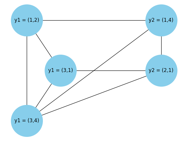
Fig. 40 Dual graph of a small CSP consisting of three variables \(X_1\), \(X_2\), and \(X_3\) each having domain \(\{1,2,3,4\}\), and two constraints \(C_1(X_1,X_2)\), \(C_2(X_2,X_3)\) having scopes \(\{X_1, X_2\}\) and \(\{X_2, X_3\}\) respectively.

You can use Ocean’s dwave_networkx to create a QUBO from the maximum independent set of the conflict graph:

>>> import dwave_networkx as dnx
>>> import networkx as nx
>>> import dimod
...
>>> G = nx.Graph()
>>> G.add_nodes_from({"y1 = (1,2)", "y1 = (3,1)", "y1 = (3,4)", "y2 = (1,4)",
...                   "y2 = (2,1)"})
>>> G.add_edges_from({("y1 = (1,2)", "y1 = (3,1)"), ("y1 = (1,2)", "y1 = (3,4)"),
...                   ("y1 = (1,2)", "y2 = (1,4)"), ("y1 = (3,1)", "y1 = (3,4)"),
...                   ("y1 = (1,2)", "y1 = (3,4)"), ("y1 = (3,1)", "y2 = (2,1)"),
...                   ("y1 = (3,4)", "y2 = (1,4)"), ("y1 = (3,4)", "y2 = (2,1)"),
...                   ("y2 = (1,4)", "y2 = (2,1)")})
>>> Q = dnx.algorithms.independent_set.maximum_weighted_independent_set_qubo(G)

Solutions to the QUBO meet the constraints (\(y_1=(1,2), y_2=(2,1)\) and \(y_1=(3,1), y_2=(1,4)\)):

>>> print(dimod.ExactSolver().sample_qubo(Q).lowest())            
  y1 = (1,2) y1 = (3,1) y1 = (3,4) y2 = (1,4) y2 = (2,1) energy num_oc.
0          1          0          0          0          1   -2.0       1
1          0          1          0          1          0   -2.0       1
['BINARY', 2 rows, 2 samples, 5 variables]

Further Information

• [Bac2002] discusses advantages and disadvantages of dual variables in modeling CSPs.

• [Fra1989] addresses the equivalence of binary and non-binary CSPs and discusses two methods of converting between these formulations through dual and hidden transformations.

Constraints: Soft/Hard (Conflict-Graph Technique)

Many CSPs used in applications are formulated with two types of constraints:

• “Hard” constraints cannot be broken in a viable solution.

• “Soft” constraints incur a penalty if broken.

You can represent hard and soft constraints by choosing two weights \(w_H\) (large magnitude) and \(w_S\) (small magnitude) to assign to the respective constraints. You then use the technique of Constraints (Conflict-Graph Technique) but in the resulting graph find a maximum independent set of minimum weight: a weighted MIS.

The QUBO representation of weighted MIS for a graph \(G=(V,E)\) is simply \(\min_\vc{x} \bigl\{ \sum_v w_v x_v + M\sum_{(v,v')\in E} x_v x_{v'} \bigr\}\) where \(w_v\) is the weight of vertex \(v\).

Ocean’s dwave_networkx lets you set a weight attribute in the example of Constraints (Conflict-Graph Technique), as shown here:

>>> import dwave_networkx as dnx
>>> import networkx as nx
>>> import dimod
...
>>> G = nx.Graph()
>>> G.add_nodes_from(["y1 = (1,2)", "y1 = (3,1)", "y1 = (3,4)"], weight=3)
>>> G.add_nodes_from(["y2 = (1,4)", "y2 = (2,1)"], weight=1)
>>> G.add_edges_from({("y1 = (1,2)", "y1 = (3,1)"), ("y1 = (1,2)", "y1 = (3,4)"),
...                   ("y1 = (1,2)", "y2 = (1,4)"), ("y1 = (3,1)", "y1 = (3,4)"),
...                   ("y1 = (1,2)", "y1 = (3,4)"), ("y1 = (3,1)", "y2 = (2,1)"),
...                   ("y1 = (3,4)", "y2 = (1,4)"), ("y1 = (3,4)", "y2 = (2,1)"),
...                   ("y2 = (1,4)", "y2 = (2,1)")})
>>> Q = dnx.algorithms.independent_set.maximum_weighted_independent_set_qubo(G,
...                                         weight="weight")

Best solutions to the QUBO still meet both constraints (first two rows with energy \(-1.333333\)), but notice the difference in energies for solutions that meet just the first constraint (rows three to five with energy \(-1.0\)) versus solutions that meet just the second constraint (last two rows with energy \(-0.333333\)):

>>> print(dimod.ExactSolver().sample_qubo(Q).lowest(atol=1.1))  
   y1 = (1,2) y1 = (3,1) y1 = (3,4) y2 = (1,4) y2 = (2,1)    energy num_oc.
12          0          1          0          1          0 -1.333333       1
30          1          0          0          0          1 -1.333333       1
1           1          0          0          0          0      -1.0       1
3           0          1          0          0          0      -1.0       1
7           0          0          1          0          0      -1.0       1
15          0          0          0          1          0 -0.333333       1
31          0          0          0          0          1 -0.333333       1
['BINARY', 7 rows, 7 samples, 5 variables]

Using this technique on real-world problems with many constraints and probabilistic solvers, such as D-Wave quantum computers, results in a higher likelihood of finding solutions that at least meet the more heavily weighted, “hard” constraints.

Constraints: Linear Equality (Penalty Functions)

You can express \(m\) equality constraints on \(n\) Boolean variables, \(\vc{x}\), as \(\vc{C}\vc{x}=\vc{c}\), where \(\vc{C}\) is an \(m\times n\) matrix and \(\vc{c}\) an \(m\times 1\) vector. Mapping these constraints to QUBO formulation, the penalty function \(\vc{C}\vc{x}-\vc{c}=0\) is simply \(M \|\vc{C}\vc{x}-\vc{c}\|^2\). For \(k\) independently weighted constraints, the penalty function in QUBO formulation is

\[P_=(\vc{x}) = \sum_k m^=_k \bigl(\ip{\vc{C}_k}{\vc{x}}-c_k \bigr)^2,\]

where \(m_k^=>0\) is the weight of the equality constraint \(k\), and \(\vc{C}_k\) is row \(k\) of \(\vc{C}\). This function is nonnegative and equal to zero for feasible \(\vc{x}\).

Example

This simple example solves the problem of finding a maximum independent set (MIS), where the graph is a Chimera cell,

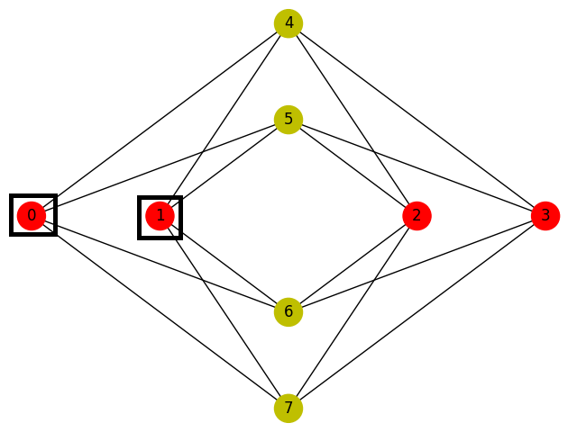
Fig. 41 A Chimera unit cell with two maximum independent sets.

but with an added constraint that requires that either node 0 or node 1, but not both, be selected. (The example in the CSP (Inverse Verification Technique) solves it by reformulating the constraint as a Boolean gate.)

You can express this \(m=1\) constraint as \(x_0 + x_1 = 1\), an equality that holds only if either but not both of its variables \(x_0, x_1\) is 1, or in the mathematical formalism of this section, \(\vc{C}\vc{x}=\vc{c}\), as:

\[\begin{split}\begin{bmatrix} 1 & 1 & 0 & 0 & 0 & 0 & 0 & 0\end{bmatrix} \begin{bmatrix} x_0 \\ x_1 \\ x_2 \\ x_3 \\ x_4\\ x_5\\ x_6 \\ x_7 \end{bmatrix} = \begin{bmatrix} 1 \\ 0 \\ 0 \\ 0 \\ 0 \\ 0 \\ 0 \\ 0 \end{bmatrix}\end{split}\]

where the \(x_i\) variables represent the graph nodes, with a value of 1 signifying that the variable belongs to the MIS.

The penalty function for the constraint in QUBO formulation is

\[ \begin{align}\begin{aligned}P_= (\vc{x}) &= (x_0 + x_1 -1)^2\\&= 2x_0x_1 -x_0 -x_1 +1\end{aligned}\end{align} \]

Dropping the constant term, which is added equally to all values of \(x_0, x_1\) and so does not favor any, you can see the penalty favors states where one and only one of the two nodes are selected:

\(x_0, x_1\)	Penalty
0, 0	0
0, 1	-1
1, 0	-1
1, 1	0

You can use Ocean’s dwave_networkx for the MIS QUBO. The code below combines the MIS and penalty QUBOs, weighting the constraint at 1.5 so the penalty for breaking this (hard) constraint is a bit higher than flipping a variable.

>>> import dwave_networkx as dnx
>>> import dimod
>>> # Create a BQM for the MIS
>>> G = dnx.chimera_graph(1, 1, 4)
>>> Q_mis = dnx.algorithms.independent_set.maximum_weighted_independent_set_qubo(G)
>>> bqm = dimod.BQM.from_qubo(Q_mis)
>>> # Create a BQM for the constraint
>>> Q_constraint = {(0, 0): -1, (1, 1): -1, (0, 1): 2}
>>> bqm_constraint = dimod.BQM.from_qubo(Q_constraint)
>>> bqm_constraint.scale(1.5)
>>> # Create a combined BQM
>>> bqm.update(bqm_constraint)
>>> # Print the best solutions
>>> print(dimod.ExactSolver().sample(bqm).lowest(atol=0.8))
   0  1  2  3  4  5  6  7 energy num_oc.
1  1  0  1  1  0  0  0  0   -4.5       1
3  0  1  1  1  0  0  0  0   -4.5       1
0  0  0  0  0  1  1  1  1   -4.0       1
2  1  1  1  1  0  0  0  0   -4.0       1
['BINARY', 4 rows, 4 samples, 8 variables]

The two best solutions meet the constrained MIS problem while the next two, with higher energy, solve the unconstrained MIS problem.

Further Information

• [Che2021] compares performance of a one-hot constraint and a wall-domain formulation.

• [Dec2003] discusses constraint programming as a declarative framework for modeling problems that require solutions to satisfy a number of constraints.

• [Ven2015b] discusses the use of penalties versus rewards for constraints.

• [Yur2022] introduces a hybrid classical-quantum framework based on the Frank-Wolfe algorithm for solving quadratic, linearly-constrained, binary optimization problems.

Constraints: Linear Inequality (Penalty Functions)

For inequality constraints of the form \(\vc{D}\vc{x}\le \vc{d}\), which are slightly more complex than linear equality constraints you can reduce the inequalities to equalities by introducing slack variables.

The inequality constraint \(\ip{\vc{D}_i}{\vc{x}}-d_i \le 0\), where \(\vc{D}_i\) is row \(i\) of \(\vc{D}\), can be rewritten as the equality \(\ip{\vc{D}_i}{\vc{x}}-d_i +\xi_i = 0\) by introducing a nonnegative slack variable \(\xi_i\ge 0\).

The slack variable may need to take a value as large as \(d_i-\min_{\vc{x}} \ip{\vc{D}_i}{\vc{x}} = d_i-\sum_j \min(D_{i,j},0)\). This slack quantity may be naively represented with \(\lceil d_i-\sum_j \min(D_{i,j},0) \rceil\) bits (i.e., to represent slack quantities up to 5, you can use 5 bits, with one bit representing 1, one bit 2, etc). However, you can also use a more concise representation, \(\xi_i = \ip{\vc{2}}{\vc{a}_i}\) where \(\vc{a}_i\) is the binary representation of \(\xi_i\), and \(\vc{2}\) is a vector whose elements are the powers of 2. This binary representation enforces the requirement that \(\xi_i\ge 0\).

Inequality \(i\) may be enforced with the penalty \(\bigl(\ip{\vc{D}_i}{\vc{x}}-d_i + \ip{\vc{2}}{\vc{a}_i}\bigr)^2\) and all constraints can be represented by summing individual inequality penalties with independent weights \(m_i^\le\) as

\[P_\le(\vc{x},\vc{a}) = \sum_i m_i^\le \bigl(\ip{\vc{D}_i}{\vc{x}}-d_i + \ip{\vc{2}}{\vc{a}_i}\bigr)^2,\]

where \(\vc{a}\) is the vector collecting all binary slack variables.

dimod can automate such reduction for you. For example, the add_linear_inequality_constraint() method below adds a constraint, \(1 \le \sum_{i=0}^{1} x_i \le 2\), that at least one of its two binary variables \(x_0, x_1\) take value one in the best solution.

>>> import dimod
>>> bqm = dimod.BinaryQuadraticModel("BINARY")
>>> slacks = bqm.add_linear_inequality_constraint([(f"x{i}", 1) for i in range(2)],
...     lagrange_multiplier=1, label="min1", lb=1, ub=2)

Example

The example of Constraints: Linear Equality (Penalty Functions) solved the problem of finding a maximum independent set (MIS), where the graph is a Chimera cell, with an equality constraint, \(x_0 + x_1 = 1\), which requires that either node 0 or node 1, but not both, be selected. Because one of those two nodes had to be selected, the equality constraint forces a selection of the MIS \(0/1, 2, 3\) (either 0 or 1, and both of 2 and 3) and not the alternative MIS \(4, 5, 6, 7\).

This example uses \(m=2\) inequality constraints to select either one of two nodes or neither:

• \(x_0 + x_1 \leq 1\)

• \(x_4 + x_5 \leq 1\)

With the above two inequality constraints the constrained MIS can be either \(0/1, 2, 3\) or \(4/5, 6, 7\).

You can now use slack variables to transform the inequalities into equalities:

\[ \begin{align}\begin{aligned}P_\le(\vc{x}, a_0) &= (x_0 + x_1 + a_0 - 1)^2\\&= 2x_0x_1 + 2x_0a_0 + 2x_1a_0 -x_0 -x_1 - a_0 +1\\P_\le(\vc{x}, a_1) &= (x_4 + x_5 + a_1 - 1)^2\\&= 2x_4x_5 + 2x_4a_1 + 2x_5a_1 -x_4 -x_5 - a_1 +1\end{aligned}\end{align} \]

where slack variables \(a_0, a_1\) can take values 0 or 1.

Table 16 shows that a relative penalty is applied to the case of \(x_0 = x_1 = 1\) or \(x_4 + x_5 = 1\) when this penalty function is minimized (when this function is part of a BQM being minimized, its value is lowest for at least one of the possible values of ancillary variable \(a_0\) or \(a_1\)). In this table, column \(\vc{x}\) is all possible states of \(x_0,x_1\) or \(x_4, x_5\); column \(\mathbf{P_{a=0}}\) and \(\mathbf{P_{a=1}}\) are the values of the penalty function if the ancillary variable \(a_0/a_1=0\) or \(a_0/a_1=1\) respectively; and the final column, \(\mathbf{\min_{a}P}\), is the value the penalty function adds to the minimized BQM (the minimum penalty of \(\mathbf{P_{a=0}}\) or \(\mathbf{P_{a=1}}\)).

Table 16 Penalty for Inequality Constraints.

\(\vc{x}\)	\(\mathbf{P_{a=0}}\)	\(\mathbf{P_{a=1}}\)	\(\mathbf{\min_{a}P}\)
\(0,0\)	\(0\)	\(-1\)	\(-1\)
\(0,1\)	\(-1\)	\(0\)	\(-1\)
\(1,0\)	\(-1\)	\(0\)	\(-1\)
\(1,1\)	\(0\)	\(3\)	\(0\)

As in the previous section, you can use Ocean’s dwave_networkx for the MIS QUBO. The code below combines the MIS and penalty QUBOs, weighting the constraint at 1.5 so the penalty for breaking these (hard) constraints is a bit higher than flipping a variable.

>>> import dwave_networkx as dnx
>>> import dimod
>>> # Create a BQM for the MIS
>>> G = dnx.chimera_graph(1, 1, 4)
>>> Q_mis = dnx.algorithms.independent_set.maximum_weighted_independent_set_qubo(G)
>>> bqm = dimod.BQM.from_qubo(Q_mis)
>>> # Create BQMs for the constraints
>>> Q_constraint1 = {(0, 0): -1, (1, 1): -1, ('a0', 'a0'): -1,
...                  (0, 1): 2, (0, 'a0'): 2, (1, 'a0'): 2}
>>> Q_constraint2 = {(4, 4): -1, (5, 5): -1, ('a1', 'a1'): -1,
...                  (4, 5): 2, (4, 'a1'): 2, (5, 'a1'): 2}
>>> bqm_constraint1 = dimod.BQM.from_qubo(Q_constraint1)
>>> bqm_constraint1.scale(1.5)
>>> bqm_constraint2 = dimod.BQM.from_qubo(Q_constraint2)
>>> bqm_constraint2.scale(1.5)
>>> # Create a combined BQM
>>> bqm.update(bqm_constraint1)
>>> bqm.update(bqm_constraint2)
>>> # Print the best solutions
>>> print(dimod.ExactSolver().sample(bqm).lowest(atol=0.8))
   0  4  5  6  7  1  2  3 a0 a1 energy num_oc.
0  0  0  1  1  1  0  0  0  1  0   -6.0       1
2  0  1  0  1  1  0  0  0  1  0   -6.0       1
3  0  0  0  0  0  1  1  1  0  1   -6.0       1
5  1  0  0  0  0  0  1  1  0  1   -6.0       1
1  0  1  1  1  1  0  0  0  1  0   -5.5       1
4  1  0  0  0  0  1  1  1  0  1   -5.5       1
['BINARY', 6 rows, 6 samples, 10 variables]

The four best solutions meet the constrained MIS problem,

• {5, 6, 7} selects 5, not 4, and neither 0 nor 1

• {4, 6, 7} selects 4, not 5, and neither 0 nor 1

• {1, 2, 3} selects 1, not 0, and neither 4 nor 5

• {0, 2, 3} selects 0, not 1, and neither 4 nor 5

while the next two, with higher energy, solve the unconstrained MIS problem.

Constraints: Nonlinear (Penalty Functions)

The previous sections show how penalty functions for equality and inequality constraints may be constructed, with inequality constraints requiring ancillary variables.

Given sets of feasible \(F\) and infeasible \(\overline{F}\) configurations, and a requirement that \(\min_{\vc{a}} P(\vc{x},\vc{a}) = o\) for \(\mathbf{x}\in F\) and \(\min_{\vc{a}} P(\mathbf{x},\vc{a}) \ge o+1\) for \(\mathbf{x}\in \overline{F}\) for some constant \(o\) representing the objective value of feasible configurations, you can formulate a quadratic penalty as

\[\begin{split}P(\vc{x},\vc{a}) = \begin{bmatrix} \vc{x} & \vc{a} \end{bmatrix} \begin{bmatrix} \vc{Q}^{x,x} & \vc{Q}^{x,a} \\ 0 & \vc{Q}^{a,a} \end{bmatrix} \begin{bmatrix} \vc{x} \\ \vc{a} \end{bmatrix}\end{split}\]

with

\[\vc{Q}^{x,x} = \sum_i w_i^{x,x} \vc{M}_i^{x,x}, \qquad \vc{Q}^{x,a} = \sum_i w_i^{x,a} \vc{M}_i^{x,a}, \qquad \vc{Q}^{a,a} = \sum_i w_i^{a,a} \vc{M}_i^{a,a}.\]

For Boolean indicator variables \(\{\alpha_k(j)\}\) for each \(1 \le j \le |F|\) and for each allowed configuration \(\vc{a}_k\) you then have

\[\begin{split}\langle \vc{1}, \vc{\alpha}(j)\rangle = 1 \quad \forall j\in F \\ \sum_{k'} \bigl\{ \langle \alpha_{k'}(j) \vc{w}^{x,a}, \vc{c}^{x,a}_{k'}(j) \rangle + \langle \alpha_{k'}(j) \vc{w}^{a,a}, \vc{c}^{a,a}_{k'} \rangle \bigr\} \le \langle \vc{w}^{x,a}, \vc{c}^{x,a}_k(j) \rangle + \langle \vc{w}^{a,a}, \vc{c}^{a,a}_k\rangle \quad \forall k,j.\end{split}\]

To break the coupling of \(\alpha_k(j)\) to \(\vc{w}^{x,a}\) and \(\vc{w}^{a,a}\) and obtain a linear problem, introduce \(\vc{v}_k^{x,a}(j) = \alpha_k(j) \vc{w}^{x,a}\) and \(\vc{v}_k^{a,a}(j) = \alpha_k(j) \vc{w}^{a,a}\). This requirement is enforced with

\[\begin{split}\vc{v}_k^{x,a}(j) &\le \alpha_k(j) \\ \vc{v}_k^{a,a}(j) &\le \alpha_k(j) M \\ -\vc{v}_k^{x,a}(j) &\le \alpha_k(j) M \\ -\vc{v}_k^{a,a}(j) &\le \alpha_k(j) M \\ \sum_k \vc{v}_k^{x,a}(j) &= \vc{w}^{x,a} \\ \sum_k \vc{v}_k^{a,a}(j) &= \vc{w}^{a,a}.\end{split}\]

The resulting mixed integer program can then be solved with any MIP solver. If there is no feasible solution for a given number of ancillary variables or specified connectivity, then these requirements must be relaxed by introducing additional ancillary variables of additional connectivity.

Further Information

• [Qui2021] transforms to QUBOs the constrained combinatorial optimization (COPT) problem of maximum k-colorable subgraph (MkCS) with its linear constraints stated as (1) linear constraints and (2) nonlinear equality constraints.

CSP (Inverse Verification Technique)

One approach to solving a constraint satisfaction problem (CSP), \(C(\vc{x}) \equiv \bigwedge_{\alpha=1}^{|\mathcal{C}|} C_\alpha(\vc{x}_\alpha)\), exploits the fact that NP-hard decision problems can be verified in polynomial time. If the CSP corresponding to \(C(\vc{x})\) is in NP, you can write the output \(z \Leftrightarrow C(\vc{x})\) as a Boolean circuit whose size is polynomial in the number of Boolean input variables. The Boolean circuit \(z\Leftrightarrow C(\vc{x})\) can be converted to an optimization objective using Boolean operations formulated as QUBO penalty functions, with each gate contributing the corresponding penalty function—see Elementary Boolean Operations.

The resulting optimization objective—which also has a polynomial number of variables and at a feasible solution \(\vc{x}^\star\), \(z_\star=1\) evaluates to 0—may be run in reverse to infer inputs from the desired true output.

To accomplish this, clamp the output of the circuit to \(z=1\) by adding \(-Mz\) (for sufficiently large \(M\)) to the objective, and then minimize with respect to all variables.[13] If you obtain a solution for which the objective evaluates to 0, you have a feasible solution to the CSP.

[13]

Alternatively, substitute \(z=1\) into the objective and eliminate \(z\) from the problem.

Example

The example of Constraints: Linear Equality (Penalty Functions) solved the problem of finding a maximum independent set (MIS), where the graph is a Chimera cell, with an equality constraint, \(x_0 + x_1 = 1\), which requires that either node 0 or node 1, but not both, be selected. (Because one of those two nodes has to be selected, the equality constraint forces a selection of the constrained MIS \(0, 2, 3\) or \(1, 2, 3\) and not the unconstrained MIS \(4, 5, 6, 7\).) That example converted the constraint into a QUBO by squaring the subtraction of the equation’s right side from the left.

This example solves the same problem but converts the constraint into a Boolean gate, in this case, the XOR gate.

You can mathematically formulate a QUBO for the XOR gate as shown in Elementary Boolean Operations; this example use Ocean’s dimod for the XOR QUBO. The code below combines the MIS and penalty QUBOs, weighting the XOR constraint at 1.5 so the penalty for breaking this (hard) constraint is a bit higher than flipping a variable, and setting \(z\) to a negative value substantially lower than other linear biases.

>>> import dwave_networkx as dnx
>>> import dimod
>>> from dimod.generators import xor_gate
>>> # Create a BQM for the MIS
>>> G = dnx.chimera_graph(1, 1, 4)
>>> Q_mis = dnx.algorithms.independent_set.maximum_weighted_independent_set_qubo(G)
>>> bqm = dimod.BQM.from_qubo(Q_mis)
>>> # Create a BQM for the constraint
>>> bqm_xor = xor_gate(0, 1, 'z', 'aux')
>>> bqm_xor.scale(1.5)
>>> # Fix z to 1
>>> Q_fix = {('z', 'z'): -3}
>>> bqm_fix = dimod.BQM.from_qubo(Q_fix)
>>> # Create a combined BQM
>>> bqm.update(bqm_xor)
>>> bqm.update(bqm_fix)
>>> # Print the best solutions
>>> print(dimod.ExactSolver().sample(bqm).lowest(atol=0.8))   
   0  4  5  6  7  1  2  3  z aux0 aux1 energy num_oc.
0  1  0  0  0  0  0  1  1  1    0    0   -6.0       1
1  0  0  0  0  0  1  1  1  1    0    1   -6.0       1
['BINARY', 2 rows, 2 samples, 11 variables]

The two best solutions meet the constrained MIS problem

Further Information

• The dwave-examples Factoring example uses this technique to solve a factoring problem as QUBOs. It shows that this formulation yields low requirements on both connectivity and precision constraints, making it suitable for the D-Wave system.

• The Example Reformulation: Circuit Fault Diagnosis example may also benefit from this technique.

Elementary Boolean Operations

As demonstrated in the CSP (Inverse Verification Technique) section, an often useful approach to consider it to reformulate your problem using BQMs derived from Boolean operations.

Table 17 shows several constraints useful in building Boolean circuits.

Table 17 QUBO Penalty Functions for Elementary Boolean Operations

Constraint	Penalty[14]
\(z \Leftrightarrow \neg x\)	\(2xz-x-z+1\)
\(z \Leftrightarrow x_1 \vee x_2\)	\(x_1 x_2 + (x_1+x_2)(1-2z) + z\)
\(z \Leftrightarrow x_1 \wedge x_2\)	\(x_1 x_2 - 2(x_1+x_2)z +3z\)
\(z \Leftrightarrow x_1 \oplus x_2\)	\(2x_1x_2 -2(x_1+x_2)z - 4(x_1+x_2)a +4az +x_1+x_2+z + 4a\)

[14]

The XOR operator, \(\oplus\), requires the introduction of a single ancillary variable \(a\).

Example: OR Gate as a Penalty

This example shows how the Boolean OR formulation given in the Table 18 table works.

In Table 18, column \(\mathbf{x_1,x_2}\) is all possible states of the gate’s inputs; column \(\mathbf{x_1 \vee x_2}\) is the corresponding output values of a functioning gate; column \(\mathbf{P(z=x_1 \vee x_2)}\) is the value the penalty function adds to the energy of the objective function when the gate is functioning (zero, a functioning gate must not be penalized) while column \(\mathbf{P(z \ne x_1 \vee x_2)}\) is the value the penalty function adds when the gate is malfunctioning (nonzero, the objective function must be penalized with a higher energy).

Table 18 Boolean OR Constraint as a Penalty.

\(\mathbf{x_1,x_2}\)	\(\mathbf{x_1 \vee x_2}\)	\(\mathbf{P(z=x_1 \vee x_2)}\)	\(\mathbf{P(z \ne x_1 \vee x_2)}\)
\(0,0\)	\(0\)	\(0\)	\(1\)
\(0,1\)	\(1\)	\(0\)	\(1\)
\(1,0\)	\(1\)	\(0\)	\(1\)
\(1,1\)	\(1\)	\(0\)	\(3\)

For example, for the state \(x_1, x_2=1,1\) of the fourth row, when \(z=x_1 \vee x_2 = 1\),

\[x_1 x_2 + (x_1+x_2)(1-2z) + z = 1+(1+1)(1-2)+1=1-2+1=0,\]

not penalizing the valid solution, whereas for \(z \ne x_1 \vee x_2 = 0\),

\[x_1 x_2 + (x_1+x_2)(1-2z) + z = 1+(1+1)(1-0)+0=1+2+0=3,\]

adding an energy cost of \(3\) to the solution that violates the constraint.

Examples

• Section Native QPU Formulations: Ising and QUBO above derives a QUBO for an NOT gate as a constraint.

• The Example Reformulation: Circuit Fault Diagnosis example derives AND and XOR gates.

• The Non-Quadratic (Higher-Degree) Polynomials also derives an AND gate.

Further Information

• [Jue2016] provides numerous Boolean operations in the Ising model. These can be converted to QUBO penalty functions as shown in Native QPU Formulations: Ising and QUBO.

Example Reformulation: Map Coloring

The map-coloring problem is to assign a color to each region of a map such that any two regions sharing a border have different colors.

Fig. 42 Coloring a map of Canada with four colors.

A solution to a map-coloring problem for a map of Canada with four colors is shown in Figure 42.

This example is intended to demonstrate the use of the reformulations techniques of this chapter. In practice, you could simply use Ocean’s min_vertex_color() to solve the problem. Ocean documentation demonstrates solutions to the map-coloring problem in the Large Map Coloring and Map Coloring: Hybrid DQM Sampler examples. The dwave-examples GitHub repo also demonstrates solutions to the map-coloring problem. [Dwave4] describes this procedure.

Step 1: State the Objectives and Constraints

As noted in the General Guidance on Reformulating section, the first step in solving a problem is to state objectives and constraints. For this problem, the colors selected must meet two constraints:

• Each region is assigned one color only, of \(C\) possible colors.

• The color assigned to one region cannot be assigned to adjacent regions.

Any solution that meets both constraints is a good solution. Because this problem has no preferences among such good solutions, it has no objective, just constraints. (For a map problem that ranks colors—for example, it prefers to color regions in yellow rather than green—you would also formulate an objective that minimizes the use of the least preferred colors.)

Step 2: Select Variables

One approach to mathematically stating this problem is to think of the regions as variables representing the possible set of colors. What type of values should these variables represent?

To represent a set of values such as [blue, green, red, yellow] you can use various numerical schemes: integer, discrete, and binary variables. Ocean documentation’s Map Coloring: Hybrid DQM Sampler example uses discrete variables and Leap’s DQM solver; this example uses binary variables to enable solution directly on a QPU solver.

More specifically, this example maps the \(C\) possible colors to a unary encoding: represent each region by \(C\) binary variables, one for each possible color, which is set to value \(1\) if selected, while the remaining \(C-1\) variables are \(0\). These are known as one-hot variables.

Table 19 shows a unary encoding for representing colors for a map with \(C=4\) possible colors, where \(q_B\) is a variable representing blue, \(q_G\) green, \(q_R\) red, and \(q_Y\) yellow.

Table 19 Translating Color to Binary.

Color	Unary Encoding
Blue	\(q_B,q_G,q_R,q_Y = 1,0,0,0\)
Green	\(q_B,q_G,q_R,q_Y = 0,1,0,0\)
Red	\(q_B,q_G,q_R,q_Y = 0,0,1,0\)
Yellow	\(q_B,q_G,q_R,q_Y = 0,0,0,1\)

Step 3: Formulate Constraints (Constraint 1)

The first constraint is that each region is assigned one color only, of \(C\) possible colors. It is formulated here using the truth-table approach of the Native QPU Formulations: Ising and QUBO section.

Simplify the problem by first considering a two-color problem. Given \(C=2\) colors that are unary encoded as \(q_B,q_G\), the constraint is reduced to feasible states being either blue selected, \(q_B,q_G=1,0\), or green selected, \(q_B,q_G=0,1\), but not both or neither selected.

Try to fit this simple constraint to the QUBO format for two variables:

\[\text{E}(a_i, b_{i,j}; q_i) = a_B q_B + a_G q_G + b_{B,G} q_B q_G.\]

Table 20 shows all the possible states for a single-region, two-color problem. In this table, columns \(\mathbf{q_B}\) and \(\mathbf{q_G}\) are all possible states of the two variables encoding the region’s two colors; column Constraint shows whether or not the state of the variables meet the constraint that one color is selected; column \(\mathbf{\text{E}(a_i, b_{i,j}; q_i)}\) is the QUBO’s energy for each state.

Table 20 States for a Constraint Selecting One of Two Colors.

\(\mathbf{q_B}\)	\(\mathbf{q_G}\)	Constraint	\(\mathbf{\text{E}(a_i, b_{i,j}; q_i)}\)
0	0	Violates	\(0\)
0	1	Meets	\(a_G\)
1	0	Meets	\(a_B\)
1	1	Violates	\(a_B+a_G+b_{B,G}\)

QUBO coefficients to represent this constraint can be guessed from looking at Table 20 and the following considerations:

• Both colors are equally preferred, so setting \(a_B=a_G\) ensures identical energy for both states that meet the constraint (\(q_B, q_G=0,1\) and \(q_B, q_G=1,0\)).

• The state \(q_B, q_G=0,0\), which violates the constraint, has energy \(0\), so to ensure that the non-violating states have lower energy, set \(a_B = a_G < 0\).

• Having set the minimum energy to negative for the valid states, setting \(a_B+a_G+b_{B,G}=0\) for non-valid state \(q_B, q_G=1,1\) ensures that state has a higher energy.

One solution[15] is to set \(a_B=a_G=-1\) and \(b_{B,G}=2\). Setting these values for the linear and quadratic coefficients sets the minimum energy for this QUBO to \(-1\) for both valid states and zero for the states that violate the constraint; that is, this QUBO has lowest energy if just one color is selected (only one variable is \(1\)), where either color (variable \(q_B\) or \(q_G\)) has an equal probability of selection.

[15]

Getting Started with D-Wave Solvers discusses the effects of different choices of values in the section on problem scaling. See also the considerations discussed in the Imprecision of Biases section.

The two-color formulation above can be easily expanded to a three-color problem: \(C=3\) possible colors are encoded as \(q_B,q_G,q_R\). The constraint to minimize in QUBO format is

\[ \text{E}(a_i, b_{i,j}; q_i) = a_B q_B + a_G q_G + a_R q_R +b_{B,G} q_B q_G + b_{B,R} q_B q_R +b_{G,R} q_G q_R.\]

Coefficients that minimize the QUBO can be guessed by applying the previous considerations more generically. All colors are equally preferred, so set \(a_i=a\) to ensure identical energy for states that meet the constraint. Simplify by setting \(b_{i,j}=b=2\) and \(a=-1\) for a QUBO,

\[ \begin{align}\begin{aligned} \text{E}(a, b; q_i) &= a(q_B + q_G + q_R) +b(q_B q_G + q_B q_R + q_G q_R)\\&= -(q_B + q_G + q_R) +2(q_B q_G + q_B q_R + q_G q_R).\end{aligned}\end{align} \]

Table 21 enumerates all states of the constraint for three possible colors. The meanings of the columns in this table are identical to those for Table 20 above.

Table 21 States for a Constraint Selecting One of Three Colors.

\(\mathbf{q_B,q_G,q_R}\)	Constraint	\(\mathbf{\text{E}(a=-1, b=2; q_i)}\)
0,0,0	Violates	\(-(0) +2(0)=0\)
0,0,1	Meets	\(-(1) + 2(0)=-1\)
0,1,0	Meets	\(-(1) + 2(0)=-1\)
0,1,1	Violates	\(-(2) + 2(1)=0\)
1,0,0	Meets	\(-(1) + 2(0)=-1\)
1,0,1	Violates	\(-(2) + 2(1)=0\)
1,1,0	Violates	\(-(2) + 2(1)=0\)
1,1,1	Violates	\(-(3) + 2(3)=3\)

Again, the minimum energy for this QUBO is \(-1\) for valid states and higher for states that violate the constraint; that is, this QUBO has lowest energy if just one color is selected (one variable is \(1\)), where the three colors (variables) have equal probability of selection.

For the four-color map problem, the one-color-per-region constraint can likewise be simplified to a QUBO objective, with \(b_{i,j}=b=2\) and \(a_i=a=-1\),

\[ \text{E}(a, b; q_i) = -(q_B + q_G + q_R + q_Y) +2(q_B q_G + q_B q_R + q_B q_Y + q_G q_R + q_G q_Y + q_R q_Y).\]

Step 3: Formulate Constraints (Constraint 2)

The second constraint is that a color assigned to one region cannot be assigned to adjacent regions.

What degree is such a constraint’s formulation likely to have? Because the constraint acts between variable pairs representing adjacent regions, you can expect that relationships between variables are reducible to quadratic. That is, this constraint too should fit a QUBO format.

Such a QUBO should have a highest energy (a penalty) when the same colors are selected for adjacent regions. That is, if blue is selected on one side of a shared border, for example, the QUBO has higher energy if blue is also selected on the other side.

Similar to the previous constraint, start with a simplified problem of two variables: the variable for green in region \(r1\), \(q_{G}^{r1}\), and for green in adjacent region \(r2\), \(q_{G}^{r2}\). The constraint is that these variables (representing color green in adjacent regions \(r1\) and \(r2\)) not have the same value (True for both regions).

Table 22 shows all the possible states for a problem with a single color, \(c\), and two adjacent regions, \(r1, r2\). The meanings of the columns in this table are identical to those for Table 20 above.

Table 22 States for a Constraint on Color \(c\) in Adjacent Regions.

\(\mathbf{q_c^{r1}}\)	\(\mathbf{q_c^{r2}}\)	Constraint	\(\mathbf{\text{E}(a_i, b_{i,j}; q_i)}\)
0	0	Meets	\(0\)
0	1	Meets	\(a_c^{r2}\)
1	0	Meets	\(a_c^{r1}\)
1	1	Violates	\(a_c^{r1}+a_c^{r2}+b_c^{r1,r2}\)

Coefficients to represent this constraint in the two-variable QUBO,

\[ \text{E}(a_i, b_{i,j}; q_i) = a^{r1}_{c} q_{c}^{r1} + a^{r2}_{c} q_c^{r2} + b_{c}^{r1,r2} q_{c}^{r1} q_c^{r2}\]

can be derived from the following considerations:

• The state \(q_c^{r1}, q_c^{r2}=0,0\), which meets the constraint, has energy \(0\), so to ensure that other non-violating states have similar low energy, set \(a_c^{r1} = a_c^{r2} = 0\).

• Having set the minimum energy to zero for the valid states, requiring \(a_c^{r1}+a_c^{r2}+b_c^{r1, r2}>0\) for non-valid state \(q_c^{r1}, q_c^{r2}=1,1\) ensures that state has a higher energy. It also mean that \(b_c^{r1, r2}\) must be positive.

Configuring \(a^{r1}_{c} = a^{r2}_{c} = 0\) and \(b_{c}^{r1,r2} = 1\) sets a higher energy for the state \(q_{c}^{r1} = q_c^{r2}\) (color \(c\) selected in both regions), penalizing that invalid state, while leaving the valid three states with an energy of \(0\).

The sum of QUBOs for both types of constraints has lowest energy when simultaneously each region is assigned a single color and adjacent regions do not select the same colors.

Example Reformulation: Circuit Fault Diagnosis

Fault diagnosis is the combinational problem of quickly localizing failures as soon as they are detected in systems. Circuit fault diagnosis (CFD) is the problem of identifying a minimum-sized set of gates that, if faulty, explains an observation of incorrect outputs given a set of inputs.

Fig. 43 A simple circuit is shown in Figure 43.

This example is intended to demonstrate the use of the reformulations techniques of this chapter. In practice, you could use Ocean’s Boolean constraints as in the Multiple-Gate Circuit example.

A Short Digression: An Intuitive Explanation of the CFD Solution

To understand the relationship between the CFD solutions and low-energy configurations, it’s helpful to look at an even smaller example.

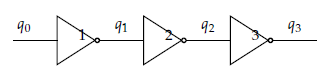
Fig. 44 The circuit in Figure 44 has three NOT gates in series, with an input \(q_0\), an output \(q_3\), and intermediate input/outputs \(q_1\) and \(q_2\).

Table 23 shows energy levels for all possible circuit states with an incorrect output for an objective function that penalizes by a value of \(1\) any malfunctioning gate.

In this table, the first column, Circuit Input (\(\mathbf{q_0}\)), is the binary input value applied to the circuit in testing, and the second column, Incorrect Output (\(\mathbf{q_3}\)), is the measured output of the circuit with an error detected. Columns \(\mathbf{q_1}\) and \(\mathbf{q_2}\) are all possible intermediate input/outputs of the circuit’s gates. Column Faulty Gate shows which gates are malfunctioning given the input and output states. Column Energy is the energy level of the objective function.

Table 23 Serial NOT Energy Levels

Circuit Input (\(\mathbf{q_0}\))	Incorrect Output (\(\mathbf{q_3}\))	\(\mathbf{q_1}\)	\(\mathbf{q_2}\)	Faulty Gate	Energy
\(0\)	\(0\)	\(0\)	\(0\)	1,2,3	\(3\)
		\(0\)	\(1\)	1	\(1\)
		\(1\)	\(0\)	3	\(1\)
		\(1\)	\(1\)	2	\(1\)
\(1\)	\(1\)	\(0\)	\(0\)	2	\(1\)
		\(0\)	\(1\)	3	\(1\)
		\(1\)	\(0\)	1	\(1\)
		\(1\)	\(1\)	1,2,3	\(3\)

The minimum-sized set of gates that, if faulty, explains the observation of incorrect outputs given a set of inputs, are the single malfunctioning gates of rows 2–7. These have the lowest non-zero energy for the serial NOT circuit.

Step 1: State the Objectives and Constraints

As noted in the General Guidance on Reformulating section, the first step in solving a problem is to state objectives and constraints. For this problem, the Boolean gates constrain outputs based on gates’ inputs; for example, the output of AND gate 1 should be \(x_1 \wedge x_2\).

The objective to be minimized is the number of faulty gates given the circuit inputs and outputs.

Good solution are those that violate the fewest of the constraints representing the circuits gates while still producing the tested inputs and outputs.

Step 2: Select Variables

The approach used in this example is to represent gate inputs and outputs with variables—the circuit is binary and so, naturally, are the variables.

Step 3: Formulate Constraints

This example maps the circuit’s gates to penalty functions using the formulations of the Elementary Boolean Operations section. These penalty functions increase the energy level of the problem’s objective function by penalizing non-valid states of the Boolean operations, which represent malfunctioning gates.

1. The NOT gate

   NOT can be represented as penalty function

   \[z \Leftrightarrow \neg x: \qquad 2xz-x-z+1.\]

   Table 24 shows that this function penalizes states that represent a malfunctioning gate while no penalty is applied to a functioning gate. In this table, column in is all possible states of the gate’s inputs; column \(\mathbf{out_{valid}}\) is the corresponding output values of a functioning gate while \(\mathbf{out_{fault}}\) is the corresponding output values of a malfunctioning gate, which are simply \(out_{fault} = \neg out_{valid}\); column \(\mathbf{P_{valid}}\) is the value the penalty function adds to the energy of the objective function when the gate is functioning (zero because a functioning gate must not be penalized) while column \(\mathbf{P_{fault}}\) is the value the penalty function adds when the gate is malfunctioning (nonzero, the objective function must be penalized with a higher energy).

   Table 24 Boolean NOT Operation as a Penalty.

   in	\(\mathbf{out_{valid}}\)	\(\mathbf{out_{fault}}\)	\(\mathbf{P_{valid}}\)	\(\mathbf{P_{fault}}\)
   \(0\)	\(1\)	\(0\)	\(0\)	\(1\)
   \(1\)	\(0\)	\(1\)	\(0\)	\(1\)

   For example, the state \(in, out_{valid}=0,1\) of the first row is represented by the penalty function with \(x=0\) and \(z = 1 = \neg x\). For this functioning gate, the value of \(P_{valid}\) is

   \[2xz-x-z+1 = 2 \times 0 \times 1 - 0 - 1 + 1 = -1+1=0,\]

   not penalizing the valid configuration. In contrast, the state \(in, out_{fault}=0,0\) of the first row is represented by the penalty function with \(x=0\) and \(z = 0 \ne \neg x\). For this malfunctioning gate, the value of \(P_{fault}\) is

   \[2xz-x-z+1 = 2 \times 0 \times 0 -0 -0 +1 =1,\]

   adding an energy cost of \(1\) to the incorrect configuration.

2. The AND gate

   AND can be represented as penalty function

   \[z \Leftrightarrow x_1 \wedge x_2: \qquad x_1 x_2 - 2(x_1+x_2)z +3z.\]

   Table 25 shows that this function penalizes states that represent a malfunctioning gate while no penalty is applied to a functioning gate. The meanings of the columns in this table are identical to those for the NOT gate above.

   Table 25 Boolean AND Operation as a Penalty.

   in	\(\mathbf{out_{valid}}\)	\(\mathbf{out_{fault}}\)	\(\mathbf{P_{valid}}\)	\(\mathbf{P_{fault}}\)
   \(0,0\)	\(0\)	\(1\)	\(0\)	\(3\)
   \(0,1\)	\(0\)	\(1\)	\(0\)	\(1\)
   \(1,0\)	\(0\)	\(1\)	\(0\)	\(1\)
   \(1,1\)	\(1\)	\(0\)	\(0\)	\(1\)

3. The XOR gate

   XOR can be represented as penalty function

   \[z \Leftrightarrow x_1 \oplus x_2: \qquad 2x_1x_2 -2(x_1+x_2)z - 4(x_1+x_2)a +4az +x_1+x_2+z + 4a,\]

   where \(a\) is an ancillary variable as described in the Non-Quadratic (Higher-Degree) Polynomials section (and shown below).

   Table 26 shows that no penalty is applied to a functioning gate when this penalty function is minimized (when this function is part of an objective function being minimized, its value is zero for at least one of the possible values of ancillary variable \(a\)). In this table, column in is all possible states of the gate’s inputs \(x_1,x_2\); column \(\mathbf{out}\) is the corresponding output values of a functioning gate \(x_1 \oplus x_2\); columns \(\mathbf{P_{a=0}}\) and \(\mathbf{P_{a=1}}\) are the values of the penalty function if the ancillary variable \(a=0\) or \(a=1\) respectively; and the final column, \(\mathbf{\min_{a}P}\), is the value the penalty function adds to the minimized objective function (the minimum penalty of \(\mathbf{P_{a=0}}\) or \(\mathbf{P_{a=1}}\)).

   Table 26 Boolean XOR Operation as a Penalty: Functioning Gate.

   in	\(\mathbf{out}\)	\(\mathbf{P_{a=0}}\)	\(\mathbf{P_{a=1}}\)	\(\mathbf{\min_{a}P}\)
   \(0,0\)	\(0\)	\(0\)	\(4\)	\(0\)
   \(0,1\)	\(1\)	\(0\)	\(4\)	\(0\)
   \(1,0\)	\(1\)	\(0\)	\(4\)	\(0\)
   \(1,1\)	\(0\)	\(4\)	\(0\)	\(0\)

   Table 27 shows that a non-zero penalty is applied to a malfunctioning gate. In this table, column \(\mathbf{out}\) is the output values of a malfunctioning gate \(out = \neg (x_1 \oplus x_2)\); the other columns are identical to those for Table 26 above.

   Table 27 Boolean XOR Operation as a Penalty: Malfunctioning Gate.

   in	\(\mathbf{out}\)	\(\mathbf{P_{a=0}}\)	\(\mathbf{P_{a=1}}\)	\(\mathbf{\min_{a}P}\)
   \(0,0\)	\(1\)	\(1\)	\(9\)	\(1\)
   \(0,1\)	\(0\)	\(1\)	\(1\)	\(1\)
   \(1,0\)	\(0\)	\(1\)	\(1\)	\(1\)
   \(1,1\)	\(1\)	\(1\)	\(1\)	\(1\)

Normalizing the Penalty Functions

To solve the CFD problem by finding a minimum-sized set of faulty gates, a search for lowest energy levels of the objective function should identify all single faults. However, if functions impose different penalties for faulty states—if some faults are penalized to a higher value than others—two faults with low penalties might produce a lower energy level than a strongly penalized single fault.

The penalty functions of the previous section impose a penalty of \(1\) on all gate faults with one exception: Table 25 shows that when the state \(in=0,0\) of the AND gate incorrectly outputs \(out=1\), the penalty imposed is \(P_{fault}=3\). This section aims to normalize the penalty functions; that is, to adjust the penalty functions so any single fault has an identical penalty, contributing equally to the objective function of the CFD problem.

One approach to normalizing the penalty function of the AND gate is to add a penalty function that imposes a reward on (a negative penalty to compensate for) the state \(in=0,0; out=1\) with its higher penalty value. The additional penalty function, \(P^*\), rewards this state with a negative penalty of value,

\[ \begin{align}\begin{aligned}P_{fault}(0,0;1)+ P^*(0,0;1) &= 1\\3+P^*(0,0;1) &= 1\\P^*(0,0;1) &= -2\end{aligned}\end{align} \]

Because both penalties are activated together in state \(in=0,0; out=1\), the total penalty they impose is \(1\), identical to the penalties of other single faults for the circuit’s gates.

The binary equivalence,

\[in_1,in_2,out=0,0,1 \longleftrightarrow \overline{in}_1,\overline{in}_2,out=1,1,1,\]

makes it straightforward to guess a penalty function, \(P^*\), that activates a reward of \(-2\) for the AND gate state of \(\overline{in}_1,\overline{in}_2,out=1,1,1\):

\[P^*= -2\overline{in}_1\overline{in}_2out.\]

Clearly this penalty function is non-zero only for faulty state \(in_1,in_2,out=0,0,1\), in which case it is equal to \(-2\). Adding this penalty to the problem’s objective function normalizes the penalty function for the AND operation.

For example, recalculating the penalty given as an example in the previous section, the state \(in=0,0; out_{valid}=0\) of the first row of Table 25 is represented by the penalty function with \(x_1=x_2=0\) and \(z = 0 = x_1 \wedge x_2\). For this functioning gate, the value of \(P_{valid}+P^*\) is

\[ \begin{align}\begin{aligned}&\overbrace{x_1 x_2 - 2(x_1+x_2)z +3z}^{P_{valid}} + \overbrace{-2\overline{x}_1\overline{x}_2z}^{P^*}\\&= \overbrace{0}^{P_{valid}} + \overbrace{-2 \times 1 \times 1 \times 0}^{P^*}\\&= 0,\end{aligned}\end{align} \]

not penalizing the valid solution. In contrast, the state \(in=0,0; out_{fault}=1\) of the same table row is represented by the penalty function with \(x_1=x_2=0\) and \(z = 1 \ne x_1 \wedge x_2\). For this malfunctioning gate, the value of \(P_{fault}+P^*\) is

\[ \begin{align}\begin{aligned}&\overbrace{x_1 x_2 - 2(x_1+x_2)z +3z}^{P_{fault}} + \overbrace{-2\overline{x}_1\overline{x}_2z}^{P^*}\\&= \overbrace{3}^{P_{fault}} + \overbrace{-2 \times 1 \times 1 \times 1}^{P^*}\\&= 3-2\\&= 1,\end{aligned}\end{align} \]

reducing the energy cost of the original AND gate from \(3\) to \(1\) for the incorrect configuration. For all other states, both valid and faulty, the normalizing penalty, \(P^*\), is zero and has no other affect on the penalty function for AND.

Reformulating Non-Quadratic Penalties as Quadratic

The normalizing penalty introduced in the previous section, \(P^* = -2\overline{in}_1\overline{in}_2out\), is cubic and must be reformulated as quadratic to be mapped onto the native (Ising or QUBO) quadratic formulations used by the D-Wave system.

Typically, you use a tool such as dimod.higherorder.utils.make_quadratic() to reduce the degree of your penalty function. This example reformulates the normalizing penalty function using the technique of reduction by minimum selection, as described in section Non-Quadratic (Higher-Degree) Polynomials, with the substitution,

\[axyz = aw ( x+y+z -2) \quad a<0,\]

where \(a\) is just a constant that must be negative (and for \(P^*\) equals \(-2\)), \(x,y,z\) are the relevant variables (here \(\overline{in}_1, \overline{in}_2, out\)), and \(w\) an ancillary variable[16] used by this technique to reduce the cubic term, \(xyz\), to a summation of quadratic terms (e.g., \(awx\)).

[16]

Similar to ancillary variable \(a\) used in the previous section for the penalty function of the AND gate.

Applying that to \(P^*\), with ancillary variable \(w\) of the general formula renamed to \(b\), gives \(P^q\), a quadratic formulation of the cubic normalizing penalty function:

\[P^*= -2\overline{in}_1\overline{in}_2out \quad \rightarrow P^q = -2b ( \overline{in}_1+\overline{in}_2+out -2)\]

Table 28 shows that the cubic and quadratic formulations of the normalizing penalty function produce identical results. In this table, column \(\mathbf{in_1,in_2,out}\) is all possible states of the gate’s inputs and output; column \(\mathbf{P^*}\) is the corresponding values of the cubic normalizing penalty function, \(P^*= -2\overline{in}_1\overline{in}_2out\); column \(\mathbf{P^q|_{b=0}}\) the values of the quadratic substitute if the ancillary variable \(b=0\) and column \(\mathbf{P^q|_{b=1}}\) the values if \(b=1\); column \(\mathbf{\min_{b}P^q}\) is the value the penalty function adds to the minimized objective function (the minimum penalty of \(\mathbf{P^q|_{b=0}}\) or \(\mathbf{P^q|_{b=1}}\)).

Table 28 Quadratic Normalizing Penalty Function.

\(\mathbf{in_1,in_2,out}\)	\(\mathbf{P^*}\)	\(\mathbf{P^q|_{b=0}}\)	\(\mathbf{P^q|_{b=1}}\)	\(\mathbf{\min_{b}P^q}\)
\(0,0,0\)	\(0\)	\(0\)	\(0\)	\(0\)
\(0,0,1\)	\(-2\)	\(0\)	\(-2\)	\(-2\)
\(0,1,0\)	\(0\)	\(0\)	\(2\)	\(0\)
\(0,1,1\)	\(0\)	\(0\)	\(0\)	\(0\)
\(1,0,0\)	\(0\)	\(0\)	\(2\)	\(0\)
\(1,0,1\)	\(0\)	\(0\)	\(0\)	\(0\)
\(1,1,0\)	\(0\)	\(0\)	\(4\)	\(0\)
\(1,1,1\)	\(0\)	\(0\)	\(2\)	\(0\)

Constructing an Objective Function

The (normalized) penalty functions, described in the previous sections, for the three types of gates in the example circuit are:

\[ \begin{align}\begin{aligned}P_{\text{AND}} &= \overbrace{x_1 x_2 - 2(x_1+x_2)z +3z}^{\text{Generic AND}} \overbrace{-2b (\overline{x}_1+\overline{x}_2+y_1 -2)}^{P^q}\\P_{\text{NOT}} &= 2xz-x-z+1\\P_{\text{XOR}} &= 2x_1x_2 -2(x_1+x_2)z - 4(x_1+x_2)a +4az +x_1+x_2+z + 4a\end{aligned}\end{align} \]

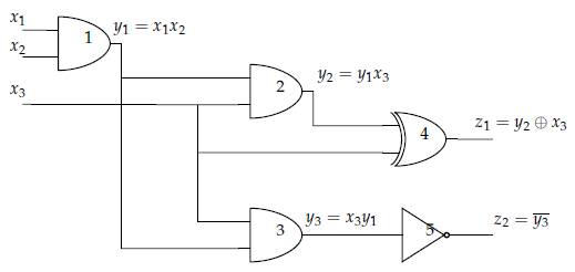
Fig. 45 The circuit for this example is shown again in Figure 45 with the output formulas of all gates also shown.

The CFD objective function is built by summing the penalty functions of all gates in the circuit:

\[ \begin{align}\begin{aligned}P_1 &= x_1 x_2 - 2(x_1+x_2)y_1 +3y_1 -2b_1 (\overline{x}_1+\overline{x}_2+y_1 -2)\\P_2 &= y_1 x_3 - 2(y_1+x_3)y_2 +3y_2 -2b_2 (\overline{y}_1+\overline{x}_3+y_2 -2)\\P_3 &= y_1 x_3 - 2(y_1+x_3)y_3 +3y_3 -2b_3 (\overline{y}_1+\overline{x}_3+y_3 -2)\\P_4 &= 2y_2x_3 -2(y_2+x_3)z_1 - 4(y_2+x_3)a +4az_1 +y_2+x_3+z_1 + 4a\\P_5 &= 2y_3z_2-y_3-z_2+1\end{aligned}\end{align} \]

where \(P_i\) is the penalty function for gate \(i\) and ancillary variables are as follows:

• \(y_i\) is the output of AND gate \(i\).

• \(a\) is the ancillary variable of the generic penalty function for XOR, used here by the penalty function for XOR gate 4.

• \(b_i\) is the ancillary variable of the generic cubic-to-quadratic reduction formula, \(b\), used here by the normalized penalty functions for AND gates 1 to 3.

A few minor adjustments can order these penalty functions in exactly the QUBO form used throughout this guide, \(\text{E}(a_i, b_{i,j}; q_i) = \sum_{i} a_i q_i + \sum_{i<j} b_{i,j} q_i q_j\).

1. Drop any freestanding constants. These do not affect the energy gap between valid and invalid configurations. In \(P_5\), for example, the \(+1\) term can be removed,

\[P_5 = 2y_3z_2-y_3-z_2\]

2. Substitute \(\neg x \Leftrightarrow (1-x)\). In \(P_1^N\), for example, use this equivalence to reformulate \(\overline{x_1}\) and \(\overline{x_2}\) introduced by \(P^*\),

\[ \begin{align}\begin{aligned}-2b_1 (\overline{x_1}+\overline{x_2}+y_1 -2) &= -2b_1 [(1-x_1) + (1-x_2) +y_1 - 2]\\&= -2b_1 (-x_1 -x_2 + y_1)\\&= 2b_1x_1 + 2b_1x_2 -2b_1y_1\end{aligned}\end{align} \]

The reordered penalty functions now have the familiar QUBO form:

\[ \begin{align}\begin{aligned}P_1 &= 3y_1 + x_1 x_2 - 2x_1y_1 +2x_1b_1 -2x_2y_1 + 2x_2b_1 -2y_1b_1\\P_2 &= 3y_2 + x_3y_1 -2x_3y_2 + 2x_3b_2 - 2y_1y_2 +2y_1b_2 -2y_2b_2\\P_3 &= 3y_3 +x_3y_1 - 2x_3y_3 + 2x_3b_3 -2y_1y_3 +2y_1b_3 -2y_3b_3\\P_4 &= x_3 + z_1 + y_2 + 4a - 2x_3z_1 + 2x_3y_2 - 4x_3a - 2z_1y_2 +4z_1a - 4y_2a\\P_5 &= -z_2 -y_3 + 2z_2y_3\end{aligned}\end{align} \]

The objective function for this CFD problem is given by,

\[\text{E}(a_i, b_{i,j}; q_i) = P_1 + P_2 + P_3 + P_4 + P_5.\]

To solve the circuit of this example, that is, to find a minimum-sized set of gates that, if faulty, explains the observation of incorrect outputs, this objective function must be minimized while holding constant the input values \(x_1,x_2,x_3=1,1,1\) and incorrect output values \(z_1,z_2=1,0\).

Example Constraints: One-Hot, Domain-Wall, \(n \choose k\)

This example solves a small, illustrative problem, a game of rock-paper-scissors, to compare two binary formulations of the one-hot constraint for discrete variables.

The rock-paper-scissors game is easily stated with discrete variables, with one variable representing the first-person player and a second representing the second-person player, with each variable having three cases: \({rock, paper, scissors}\). The winning hands are rock vs. scissors, paper vs. rock, and scissors vs. paper, and the problem is to formulate an objective function such that these hands have the lowest energy.

DQM Formulation

For reference, this example first presents a solution that exploits the high level of abstraction provided by Ocean’s DiscreteQuadraticModel and Leap’s LeapHybridDQMSampler solver.

This formulation creates a discrete quadratic model with two variables, me and you, representing two hands, each with cases rock (“R”), paper (“P”), and scissors (“S”). Negative quadratic biases are set to produce a lower value of the DQM for cases of me winning over cases of you; for example, the interaction R-S (my rock vs. your scissors) is set to -1 while S-R (my scissors vs. your rock) is set to +1.

>>> import dimod
>>> from dwave.system import LeapHybridDQMSampler
...
>>> cases = ["R", "P", "S"]
>>> win = {"R": "S", "P": "R", "S": "P"}
...
>>> dqm = dimod.DiscreteQuadraticModel()
>>> dqm.add_variable(3, label='me')
'me'
>>> dqm.add_variable(3, label='you')
'you'
>>> for my_idx, my_case in enumerate(cases):
...    for your_idx, your_case in enumerate(cases):
...       if win[my_case] == your_case:
...          dqm.set_quadratic('me', 'you',
...                            {(my_idx, your_idx): -1})
...       if win[your_case] == my_case:
...          dqm.set_quadratic('me', 'you',
...                            {(my_idx, your_idx): 1})
...
>>> dqm_sampler = LeapHybridDQMSampler()      
...
>>> sampleset = dqm_sampler.sample_dqm(dqm)   
>>> print("{} beats {}".format(cases[sampleset.first.sample['me']],
...                            cases[sampleset.first.sample['you']]))   
R beats S

BQM Formulation Using One-Hot Constraints

The basic equality-to-minimization converts an equality constraint to a minimization expression by moving all arguments and constants to one side of the equality and squaring the non-zero side of the equation. This leaves an expression that is satisfied at its smallest value (0) and unsatisfied at any larger value (>0). For example, the equation \(x+1=2\) is converted to \(\min_x[2-(x+1)]^2\), which has a minimum value of zero for the solution of the equation, \(x=1\). This same approach is used for \(n \choose k\) constraints (selection of exactly \(k\) of \(n\) variables), where you disfavor selections of greater or fewer than \(k\) variables with the penalty \(P = \alpha (\sum_{i=1}^n x_i - k)^2\), where \(\alpha\) is a weighting coefficient (see penalty method) used to set the penalty’s strength.

A one-hot constraint is therefore enforced with the penalty,

\[P = \alpha (\sum_{i=1}^n x_i - 1)^2.\]

Now, represent each player’s hand by three binary variables:

• First-person (me) player’s hand: "R", "P", "S"

• Second-person (you) player’s hand: "r", "p", "s"

For this formulation, in addition to penalizing interactions between these two hands to prefer winning to losing hands, you create one-hot constraints on each set of variables to ensure only one case (either rock or paper or scissors) is played.

>>> import dimod
>>> bqm_1hot_me = dimod.generators.combinations(["R", "P", "S"], 1)
>>> bqm_1hot_you = dimod.generators.combinations(["r", "p", "s"], 1)

You can see that lower-energy solutions to these BQMs indeed meet the one-hot constraint:

>>> print(dimod.ExactSolver().sample(bqm_1hot_me).lowest())
   P  R  S energy num_oc.
0  0  1  0    0.0       1
1  1  0  0    0.0       1
2  0  0  1    0.0       1
['BINARY', 3 rows, 3 samples, 3 variables]

Create a BQM with negative penalties for winning and positive penalties for losing (this is similar to the DQM formulation) and add the one-hot constraints, scaled as needed:

>>> bqm_game = dimod.BQM({('R', 'p'): 1, ('R', 's'): -1, ('P', 'r'): -1,
...                       ('P', 's'): 1, ('S', 'r'): 1, ('S', 'p'): -1},
...                       vartype='BINARY')
>>> bqm_1hot_me.scale(1.5)
>>> bqm_game.update(bqm_1hot_me)
>>> bqm_1hot_you.scale(1.5)
>>> bqm_game.update(bqm_1hot_you)

You can see that the lowest-energy samples meet the one-hot constraints and represent winning hands. For example, the first sampleset represents rock winning against scissors.

>>> print(dimod.ExactSolver().sample(bqm_game).lowest(atol=0.8))
   P  R  S  p  r  s energy num_oc.
0  0  1  0  0  0  1   -1.0       1
1  1  0  0  0  1  0   -1.0       1
2  0  0  1  1  0  0   -1.0       1
['BINARY', 3 rows, 3 samples, 6 variables]

Figure 46 visualizes the three combined BQMs.

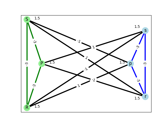
Fig. 46 A visualization of rock-paper-scissors problem using one-hot constraints: green nodes and edges represent the first-person player’s hand (me) as a one-hot BQM, blue nodes and edges represent the second-person player’s hand (you) as a one-hot BQM, and the black edges represent the penalties for winning and losing.

Notice that the one-hot constraints require that each set of binary variables representing a discrete variable be fully connected.

An embedding is shown in Figure 47.

Fig. 47 An embedding for the rock-paper-scissors problem using one-hot constraints in an Advantage QPU.

BQM Formulation Using Domain-Wall Constraints

This example formulates the discrete variables using the domain-wall encoding of [Che2021]. A one-hot constraint for discrete variable \(D_i\) is enforced with the domain-wall penalty,

\[P_i = -\kappa \sum_{u=-1}^{M-2} s_{i, u} s_{i, u+1}\]

where \(\kappa\) is a weighting coefficient (see penalty method) used to set the penalty’s strength, \(M\) is the number of cases of variable \(D_i\), and \(s_{i, -1}=-1\) and \(s_{i, M-1}=+1\) are qubits fixed to spin down and spin up, respectively, in an Ising objective function that represents a ferromagnetic chain of qubits.

Table 29 shows each term of the domain-wall penalty’s summation for the discrete variable me, with \(M=3\) cases \(rock, paper, scissors\), of this example.

Table 29 Domain-Wall Encoding for Three-Case Discrete Variable

\(u\)	\(s_{i, u}\)	\(s_{i, u+1}\)	\(s_{i, u} s_{i, u+1}\)
-1	\(s_{i, -1} = -1\)	\(s_{i, 0}\)	\(s_{i, -1} s_{i, 0} = -s_{i, 0}\)
0	\(s_{i, 0}\)	\(s_{i, 1}\)	\(s_{i, 0} s_{i, 1}\)
1	\(s_{i, 1}\)	\(s_{i, 2} =+1\)	\(s_{i, 1} s_{i, 2} = +s_{i, 1}\)

This penalty can be reordered into the standard Ising format (multiplied by \(\kappa\)):

\[ \begin{align}\begin{aligned}P_i(M=3) &= -\kappa \left( -s_{i, 0} + s_{i, 1} + s_{i, 0} s_{i, 1} \right)\\&= \kappa \left( s_{i, 0} - s_{i, 1} - s_{i, 0} s_{i, 1} \right)\end{aligned}\end{align} \]

This objective function has four possible states, three of which are ground states (lowest energy solutions), shown below for \(\kappa=1\):

>>> print(dimod.ExactSolver().sample_ising({0: 1, 1:-1}, {(0, 1): -1}))
   0  1 energy num_oc.
0 -1 -1   -1.0       1
2 +1 +1   -1.0       1
3 -1 +1   -1.0       1
1 +1 -1    3.0       1
['SPIN', 4 rows, 4 samples, 2 variables]

Figure 48 visualizes the domain walls for all possible states of the ferromagnetic chain of qubits that represent the constraint of this example.

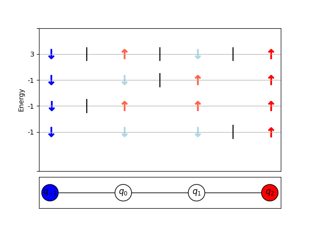
Fig. 48 A visualization of rock-paper-scissors problem using domain-walls constraint: the bottom graphic shows a ferromagnetic chain of four qubits, with qubit \(q_{-1}\) fixed to a value of spin down and qubit \(q_2\) fixed a value of spin up; the top graphic shows the qubit spins for all possible states of the chain, in four rows, with the fixed qubits in dark blue (spin down) or dark red (spin up) and non-fixed qubits in light red and blue, the consequent energies, and the domain wall or walls as a vertical black line. The low-energy states have a single domain wall; the higher energy states have more than one wall (three for this constraint).

The position of the domain wall for each state (for states that have a single domain wall only) encodes a case of the discrete variable, \(D_i\), as follows:

\[D_i = \frac{1}{2} \left( s_{i, u} - s_{i, u-1} \right) \qquad u \in [0 .. M-1]\]

Table 30 demonstrates the decoding of discrete variable me, with its \(M=3\) cases \(rock, paper, scissors\).[17]

Table 30 Domain-Wall Decoding for Three-Case Discrete Variable

\(u\)	\(s_{i, u}\)	\(s_{i, u-1}\)	\(s_{i, u} - s_{i, u-1}\)	\(D_u=1\)
0	\(s_{i, 0}\)	\(s_{i, -1} = -1\)	\(s_{i, 0} - s_{i, -1} = s_{i, 0} + 1\)	↓ ↑ ↑ ↑
1	\(s_{i, 1}\)	\(s_{i, 0}\)	\(s_{i, 1} - s_{i, 0}\)	↓ ↓ ↑ ↑
2	\(s_{i, 2} = +1\)	\(s_{i, 1}\)	\(s_{i, 2} - s_{i, 1} = 1 - s_{i, 1}\)	↓ ↓ ↓ ↑

[17]

For example, for state ↓ ↑ ↑ ↑, represented by a fixed spin down on one end of the chain (qubit -1), a fixed spin up on the other end (qubit 2), and spin up for the middle two qubits (qubits 0 and 1), the discrete variable me decodes by the \(D_{me} = \frac{1}{2} \left( s_{me, u} - s_{me, u-1} \right)\) formula to case 1 as follows:

• \(u=0\):

  \[\frac{1}{2} \left( s_{me, 0} + 1 \right) = \frac{1}{2} \left(1 + 1) \right) = \frac{1}{2} 2= 1\]

• \(u=1\):

  \[\frac{1}{2} \left( s_{me, 1} - s_{me, 0} \right) = \frac{1}{2} \left(1 -1) \right) = \frac{1}{2} 0 = 0\]

• \(u=2\):

  \[\frac{1}{2} \left( 1 - s_{me, 1} \right) = \frac{1}{2} \left(1 -1) \right) = \frac{1}{2} 0 = 0\]

The following code uses this encoding, following [Cha2019], to again solve the rock-paper-scissors problem. BQM bqm_dw represents the first-person player’s hand (me) with variables prefixed with m and the second-person player’s hand (you) with variables prefixed with y.

>>> linear = {'m0': .75, 'm1': -1.25, 'y0': 1.25, 'y1': -0.75}
>>> quadratic = {('m0', 'm1'): -1, ('y0', 'y1'): -1, ('m0', 'y1'): 0.75,
...              ('m1', 'y0'): -0.75}
>>> bqm_dw = dimod.BQM(linear, quadratic, vartype='SPIN')
>>> sampleset = dimod.ExactSolver().sample(bqm_dw).lowest(atol=0.8)

Notice that, as expected, three states are ground states:

>>> print(sampleset)
  m0 m1 y0 y1 energy num_oc.
0 +1 +1 -1 -1   -3.0       1
1 -1 +1 +1 +1   -3.0       1
2 -1 -1 -1 +1   -3.0       1
['SPIN', 3 rows, 3 samples, 4 variables]

Figure 49 visualizes the BQM.

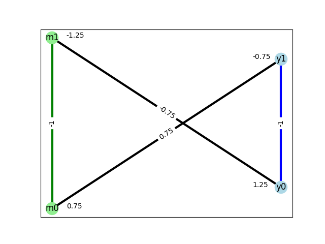
Fig. 49 A visualization of rock-paper-scissors problem using domain-wall constraints: green nodes and edges represent the first-person player’s hand (me), blue nodes and edges represent the second-person player’s hand (you), and the black edges represent the penalties for winning and losing.

Such an encoding requires fewer binary variables to represent discrete variables. Note that because the discrete variables are represented by fewer qubits than the number of cases, the problem no longer maps directly to interactions between cases as in Figure 46 of the previous subsection, with its clear separation of BQMs representing one-hot constraints and the original problem. . An embedding is shown in Figure 50.

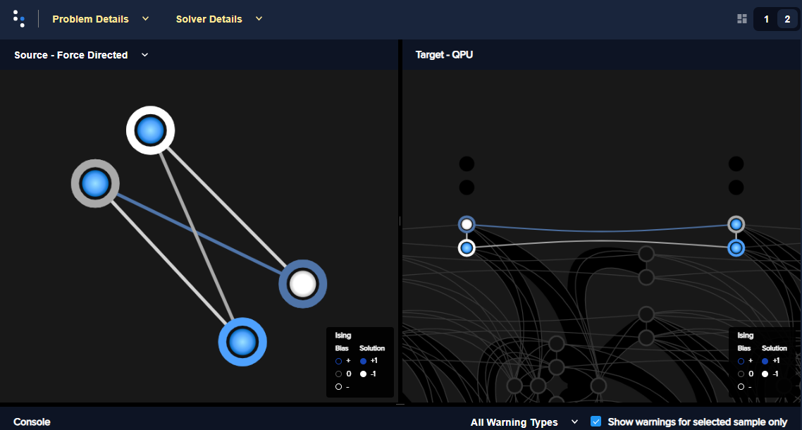
Fig. 50 An embedding for the rock-paper-scissors problem using domain-wall encoding in an Advantage QPU.

The code below maps from domain-wall encoding to the same scheme as used by the one-hot example above:

• "R", "P", "S" for the first-person player’s hand (me)

• "r", "p", "s" for the second-person player’s hand (you)

>>> ends = {'m-1': -1, 'y-1': -1, 'm2': 1, 'y2': 1}
>>> for sample in sampleset.samples():
...     solution = {}
...     chain = {**dict(sample), **ends}
...     chain_me = {int(key[1:]): val for key, val in chain.items() if 'm' in key}
...     chain_you = {int(key[1:]): val for key, val in chain.items() if 'y' in key}
...     for i, case in enumerate(['R', 'P', 'S']):
...         solution[case] = 0.5*(chain_me[i] - chain_me[i-1])
...         solution[case.lower()] = 0.5*(chain_you[i] - chain_you[i-1])
...     print(solution)                                       
{'R': 1.0, 'P': 0.0, 'S': 0.0, 'r': 0.0, 'p': 0.0, 's': 1.0}
{'R': 0.0, 'P': 1.0, 'S': 0.0, 'r': 1.0, 'p': 0.0, 's': 0.0}
{'R': 0.0, 'P': 0.0, 'S': 1.0, 'r': 0.0, 'p': 1.0, 's': 0.0}

Again the lowest-energy samples meet the one-hot constraint and represent winning hands. For example, the first sampleset represents rock winning against scissors.

\(n \choose k\) Formulation

Ocean’s dimod.generators.combinations() function can build a BQM that is minimized when exactly \(k\) of its variables equal 1.

>>> import dimod
>>> bqm_2hot = dimod.generators.combinations(["u", "v", "w"], 2)
>>> print(dimod.ExactSolver().sample(bqm_2hot).lowest())
   u  v  w energy num_oc.
0  1  1  0    0.0       1
1  0  1  1    0.0       1
2  1  0  1    0.0       1
['BINARY', 3 rows, 3 samples, 3 variables]