QPU Solvers: Configuration#
When preparing your problem for submission, consider the analog nature of quantum computers, and take measures to increase the likelihood of finding good solutions.
This chapter presents guidance on the following topics:
Read-Anneal Cycles#
The Solver Parameters section of the Getting Started with D-Wave Solvers guide explains why you should always request multiple read-anneal cycles for problems you submit to a D-Wave QPU solver.
As a guideline, equalizing your annealing and reading times is cost-effective. Increasing the number of reads can give better solutions, but improvements diminish over some problem-dependent number. If you were sampling independently from a normal distribution on energies, the sample minimum would decrease as the logarithm of the number of samples. If you were sampling from a lower-bounded distribution (e.g. containing a minimum-energy ground state), taking more samples beyond some number no longer improves the result.
Increasing both annealing time and num_reads increases your probability of success for a problem submission. The optimal combination of annealing time and number of reads to produce the best solution in a fixed time budget is problem dependent, and requires some experimentation.
Example#
This example submits the same BQM, randomly generated using the
dimod ran_r()
class and identically embedded in the same QPU, first with num_read=10000
and an anneal time of 1 \(\mu s\) and then with num_reads=1000 and an
anneal time of 50 \(\mu s\). The percentage of best solutions are compared.
>>> from dwave.system import DWaveSampler, FixedEmbeddingComposite, EmbeddingComposite
>>> qpu = DWaveSampler()
>>> import dimod
>>> import dwave.inspector
...
>>> bqm = dimod.generators.ran_r(5, 25)
>>> sampleset_1 = EmbeddingComposite(qpu).sample(bqm,
...                                              return_embedding=True,
...                                              answer_mode="raw",
...                                              num_reads=10000,
...                                              annealing_time=1)
>>> embedding = sampleset_1.info["embedding_context"]["embedding"]
>>> sampleset_50 = FixedEmbeddingComposite(qpu, embedding).sample(bqm,
...                                                               answer_mode="raw",
...                                                               num_reads=1000,
...                                                               annealing_time=50)
>>> print("Best solutions are {}% of samples.".format(
...       len(sampleset_1.lowest(atol=0.5).record.energy)/100))
Best solutions are 1.31% of samples.
>>> print("Best solutions are {}% of samples.".format(
...       len(sampleset_50.lowest(atol=0.5).record.energy)/10))
Best solutions are 4.0% of samples.
Figure 66 shows energy histograms from this example’s two submissions.
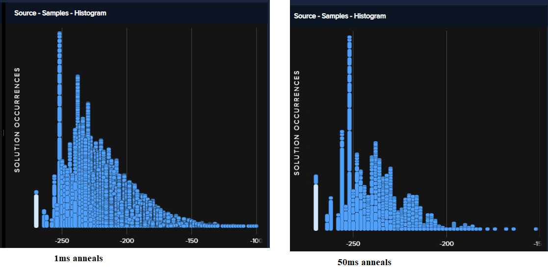
Fig. 66 Energy histograms for 10,000 samples with an anneal time of 1 \(\mu s\) (left) versus 1,000 samples with an anneal time of 50 \(\mu s\) (right).#
For this particular example, it makes sense to increase the anneal time at the expense of fewer anneal cycles (number of reads). That might not be true of other problems.
Spin-Reversal (Gauge) Transforms#
Coupling \(J_{i,j}\) adds a small bias to qubits \(i\) and \(j\) due to leakage. This can become significant for chained qubits: see integrated control errors (ICE) 1. Additionally, qubits are biased to some small degree in one direction or another due to QPU imperfections.
Applying a spin-reversal transform can improve results by reducing the impact of such unintended biases. A spin-reversal transform does not alter the Ising problem; the transform simply amounts to reinterpreting spin up as spin down, and visa-versa, for a particular spin. The technique works as follows: Given an \(n\)-variable Ising problem, we can select a random \(g\in\{\pm1\}^n\) and transform the problem via \(h_i\mapsto h_ig_i\) and \(J_{ij}\mapsto J_{ij}g_ig_j\). A spin-reversal transform does not alter the mathematical nature of the Ising problem. Solutions \(s\) of the original problem and \(s^\prime\) of the transformed problem are related by \(s^\prime_i=s_ig_i\) and have identical energies. However, the sample statistics can be affected by the spin-reversal transform because the QPU is a physical object with asymmetries.
Spin-reversal transforms work correctly with postprocessing and chains. Majority voting happens on the original problem state, not on the transformed state.
Changing too few spins leaves most errors unchanged, and therefore has little effect.
Changing too many spins means that most couplers connect spins that are both transformed, thus \(J_{i,j}\) does not change sign. As a result, some systematic errors associated with the couplers are unaffected.
Ocean software’s
SpinReversalTransformComposite composite
enables you to specify some number, num_spin_reversal_transforms, of
spin-reversal transforms for a problem. Note that increasing this number increases
the total run time of the problem.
Example#
This example solves Ocean’s AND gate example
using illustratively long chains for two of the variables (for reference, you
can embed this AND gate onto three qubits on an Advantage QPU). The first
submission does not use spin-reversal transforms while the second does.
An AND gate has four feasible states: \(x1, x2, out\) should take values
\(000, 010, 100, 111\). The example prints the percentage of samples found
for each of the feasible states of all lowest-energy samples with unbroken chains
(typically this example also produces a small number of solutions with broken
chains). Ideally, for a perfectly balanced QPU, feasible states would be
found in equal numbers: [25 25 25 25] percent.
Note
The qubits selected below for chains are available on the particular Advantage QPU used for the example. Select a suitable embedding for the QPU you run examples on.
>>> import time
>>> from dwave.system import DWaveSampler, FixedEmbeddingComposite
>>> from dwave.preprocessing import SpinReversalTransformComposite
...
>>> qpu = DWaveSampler()
>>> Q = {('x1', 'x2'): 1, ('x1', 'z'): -2, ('x2', 'z'): -2, ('z', 'z'): 3}
>>> embedding = {'x1': [2146, 2131, 2145, 2147, 3161, 3176, 3191, 3206, 3221,
...              3236,  3281, 3296, 3311, 3326], 'x2': [3251, 2071, 2086, 2101,
...              2116, 2161, 2176, 2191, 2206, 2221, 2236, 3250, 3252], 'z': [3266]}
...
>>> start_t = time.time_ns(); \
... sampleset = FixedEmbeddingComposite(qpu, embedding).sample_qubo(Q, num_reads=5000);\
... print(sampleset); \
... time_ms = (time.time_ns() - start_t)/1000000
   x1 x2  z energy num_oc. chain_b.
0   1  1  1    0.0    1226      0.0
1   0  0  0    0.0     713      0.0
2   0  1  0    0.0     957      0.0
3   1  0  0    0.0    2076      0.0
6   1  0  0    0.0       1 0.333333
7   1  0  0    0.0       5 0.333333
8   0  1  0    0.0       1 0.333333
9   1  0  0    0.0       1 0.333333
10  1  0  0    0.0       1 0.333333
11  1  0  0    0.0       1 0.333333
4   0  1  1    1.0       2      0.0
5   1  0  1    1.0      16      0.0
['BINARY', 12 rows, 5000 samples, 3 variables]
...
>>> print(time_ms)
1146.5026
...
>>> start_t = time.time_ns(); \
... sampleset_srt = FixedEmbeddingComposite(SpinReversalTransformComposite(qpu), embedding).sample_qubo(
...     Q, num_reads=500,  num_spin_reversal_transforms=10); \
... print(sampleset_srt.aggregate()); \
... time_ms = (time.time_ns() - start_t)/1000000
  x1 x2  z energy num_oc. chain_.
0  1  1  1    0.0    1519     0.0
1  0  1  0    0.0    1557     0.0
2  0  0  0    0.0     809     0.0
3  1  0  0    0.0    1090     0.0
4  1  1  0    1.0       6     0.0
5  1  0  1    1.0      12     0.0
6  0  1  1    1.0       7     0.0
['BINARY', 7 rows, 5000 samples, 3 variables]
...
>>> print(time_ms)
4231.5592
Note that the submission using spin reversals produced more balanced solutions (the four feasible configurations for an AND gate are closer to being 25% of the lowest-energy samples with unbroken chains). Note too that the runtime increased from about one second to about four seconds.
Further Information
QPU Solver Datasheet describes ICE in the D-Wave system.
[Ray2016] about temperature estimation in quantum annealers also looks at effects of spin-reversal transforms.
Postprocessing#
Postprocessing optimization and sampling algorithms provide local improvements with minimal overhead to solutions obtained from the quantum processing unit (QPU).
Ocean software provides postprocessing tools.
Example: Broken-Chain Fixing#
By default, Ocean embedding composites such as the
EmbeddingComposite class fix broken chains.
This three-variable example ferromagnetically couples variable a, represented
by a two-qubit chain, to two variables, b and c, that have opposing
biases and are represented by one qubit each. Setting a chain strength that is
smaller than the ferromagnetic coupling makes it likely for the chain to break.
Figure 67 shows the problem graph and its embedding in an Advantage QPU.
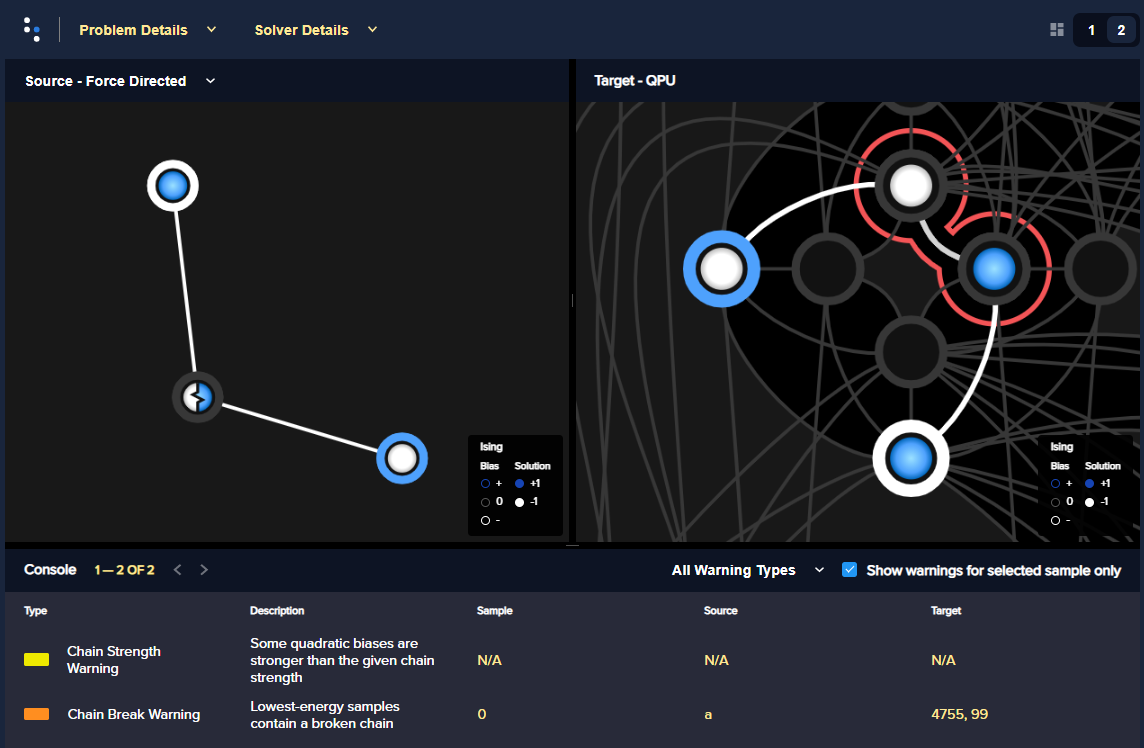
Fig. 67 The problem graph (left) and a particular embedding on a QPU (right), with a broken chain, as displayed by the problem inspector.#
The first submission uses Ocean’s default postprocessing of chains to set a
value for variable a; the second submission discards samples with broken
chains.
Note
The qubits selected below are available on the particular Advantage QPU used for the example. Select a suitable embedding for the QPU you run examples on.
>>> from dwave.system import DWaveSampler, FixedEmbeddingComposite
>>> from dwave.embedding import chain_breaks
...
>>> qpu = DWaveSampler(solver={'topology__type': 'pegasus'})
>>> embedding={'a': [4755, 99], 'b': [69], 'c': [4785]}
...
>>> sampleset = FixedEmbeddingComposite(qpu, embedding=embedding).sample_ising(
...                                     {'b': +1, 'c': -1}, {'ab': -1, 'ac': -1},
...                                     chain_strength=0.8,
...                                     num_reads=1000)
>>> print(sampleset)
   a  b  c energy num_oc. chain_b.
0 +1 -1 +1   -2.0     672 0.333333
1 -1 -1 +1   -2.0      49      0.0
2 +1 +1 +1   -2.0     118      0.0
3 -1 -1 -1   -2.0      74      0.0
4 +1 -1 +1   -2.0      87      0.0
['SPIN', 5 rows, 1000 samples, 3 variables]
...
>>> sampleset = FixedEmbeddingComposite(qpu, embedding=embedding).sample_ising(
...                                     {'b': +1, 'c': -1}, {'ab': -1, 'ac': -1},
...                                     chain_strength=0.8,
...                                     num_reads=1000,
...                                     chain_break_method=chain_breaks.discard)
>>> print(sampleset)
   a  b  c energy num_oc. chain_.
0 -1 -1 +1   -2.0      60     0.0
1 +1 +1 +1   -2.0      79     0.0
2 -1 -1 -1   -2.0     142     0.0
3 +1 -1 +1   -2.0      77     0.0
['SPIN', 4 rows, 358 samples, 3 variables]
Example: Local Search#
dwave-greedy provides an
implementation of a steepest-descent solver,
SteepestDescentSolver, for binary quadratic models.
This example runs this classical algorithm initialized from QPU samples to find minima in the samples’ neighborhoods.
>>> from dwave.system import DWaveSampler, EmbeddingComposite
>>> from greedy import SteepestDescentSolver
>>> import dimod
...
>>> solver_greedy = SteepestDescentSolver()
>>> bqm = dimod.generators.ran_r(5, 25)
>>> sampleset = EmbeddingComposite(DWaveSampler()).sample(bqm,
...                                                       num_reads=100,
...                                                       answer_mode='raw')
>>> sampleset_pp = solver_greedy.sample(bqm, initial_states=sampleset)
Figure 67 compare the results before and after the postprocessing..
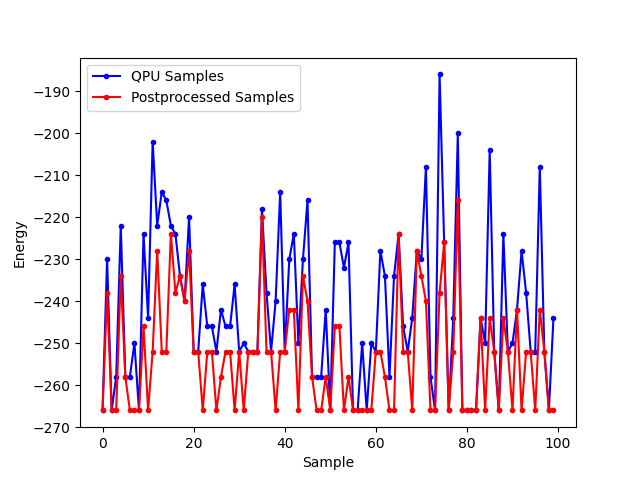
Fig. 68 Samples returned from the QPU (blue) and the samples with postprocessing (red).#
Further Information#
The Postprocessing with a Greedy Solver example in the Ocean documentation is a similar example of using
dwave-greedy, but on a native problem.
Imprecision of Biases#
Ising problems with high-precision parameters (\(h_i\) and \(J_{i,j}\)) present a challenge for quantum computers due to the finite precision available on \(\vc{h}\) and \(\vc{J}\). A problem may have lowest energy states that are sensitive to small variations in \(h\) or \(J\) while also requiring a large range of \(h\) or \(J\) values or high penalty values to enforce constraints on chains of qubits.
These are typically quantitative optimization problems rather than problems of a purely combinatorial nature (such as finding a subgraph with certain properties), where the number and connectivity of the qubits is more important than the weights, and problems for which near-optimal solutions are unacceptable. The solution’s quality depends on slight differences, at low-energy regions of the solution space, of the problem Hamiltonian as delivered to the QPU from its specification.
Example: Limiting Biases with Embedding#
You can improve results by minimizing the range of on-QPU \(J\) or \(h\) values through embeddings.
For example, if a problem variable \(s_i\), which has the largest parameter value \(h_i\), is represented by qubits \(q_i^1, q_i^2\), and \(q_i^3\) having the same value in any feasible solution, \(h_i\) can be shared across the three qubits; i.e., \(h_i s_i \rightarrow (h_i/3)(q_i^1+q_i^2+q_i^3)\), reducing \(h_i\) by a factor of 3. In a similar way, coupling parameters \(J_{i,j}\) may also be shared.
In any embedding there may be multiple edges between chains of qubits representing problem variables. You can enhance precision (at the cost of using extra qubits) by sharing the edge weight across these edges.
>>> from dwave.system import DWaveSampler, EmbeddingComposite, FixedEmbeddingComposite
>>> import networkx as nx
>>> import dimod
>>> import random
>>> import dwave.inspector
...
>>> # Create a 5-variable problem with one outsized bias
>>> G = nx.generators.small.bull_graph()
>>> for edge in G.edges:
...     G.edges[edge]['quadratic'] = random.choice([1,-1])
>>> for node in range(max(G.nodes)):
...    G.nodes[node]['linear'] = random.choice([0.1,-0.1])
>>> G.nodes[max(G.nodes)]['linear'] = 10
>>> bqm = dimod.from_networkx_graph(G,
...                                 vartype='SPIN',
...                                 node_attribute_name ='linear',
...                                 edge_attribute_name='quadratic')
>>> # Submit the problem to a QPU solver
>>> qpu = DWaveSampler(solver={'topology__type': 'pegasus'})
>>> sampleset = EmbeddingComposite(qpu).sample(bqm, num_reads=1000, return_embedding=True)
Figure 70 shows the embedded problem with the large-biased variable represented by qubit 3999.
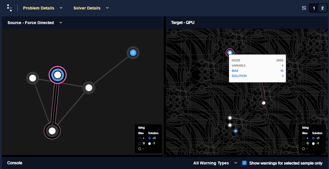
Fig. 69 An embedded problem with one large-biased variable.#
>>> embedding = dict(sampleset.info["embedding_context"]["embedding"])
>>> embedding[4]
(3999,)
>>> embedding[4] = [3999, 1715, 1730, 1745]
>>> sampleset = FixedEmbeddingComposite(qpu, embedding).sample(bqm, num_reads=1000)
Figure 70 shows the embedded problem with the large-biased variable represented by four chained qubits.
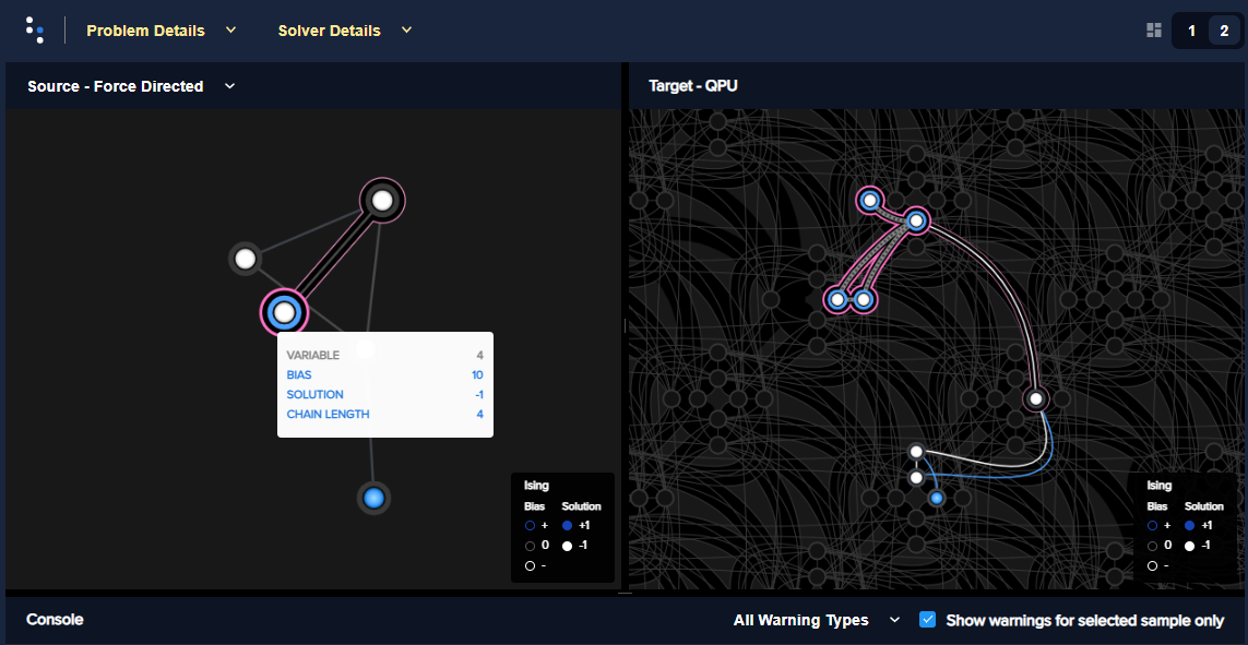
Fig. 70 A large-biased variable represented by four chained qubits.#
Example: Limiting Biases by Simplifying the Problem#
In problems with interaction \(h_i s_i\), where \(h_i>0\) is much larger than all other problem parameters, it is likely that in low-energy states, \(s_i=-1\) (\(2h\) lower in energy than \(s_i=+1\)). Generally, you may be able to identify, in polynomial time, a subset of variables that always take the same value in the ground state. You can then eliminate such variables from the problem.
Consider preprocessing problems to determine whether certain variable values can be inferred. There is little overhead in attempting to simplify every problem before sending it to the QPU.
The code below preprocesses the problem of the previous section, which has a
single outsized value for variable 4.
>>> from dwave.system import DWaveSampler, EmbeddingComposite
>>> import networkx as nx
>>> import dimod
>>> import random
>>> from dwave.preprocessing import FixVariablesComposite
...
>>> # Create a 5-variable problem with one outsized bias
>>> G = nx.generators.small.bull_graph()
>>> for edge in G.edges:
...     G.edges[edge]['quadratic'] = random.choice([1,-1])
>>> for node in range(max(G.nodes)):
...    G.nodes[node]['linear'] = random.choice([0.1,-0.1])
>>> G.nodes[max(G.nodes)]['linear'] = 10
>>> bqm = dimod.from_networkx_graph(G,
...                                 vartype='SPIN',
...                                 node_attribute_name ='linear',
...                                 edge_attribute_name='quadratic')
>>> # Preprocess and submit to a QPU solver
>>> sampler_pp = FixVariablesComposite(EmbeddingComposite(DWaveSampler()), algorithm="roof_duality")
>>> sampleset = sampler_pp.sample(bqm, num_reads=1000, return_embedding=True)
The problem submitted to the QPU has had the value of variable 4 fixed by
the FixVariablesComposite
composite using the roof duality algorithm.
Further Information#
[Kin2014] discusses preprocessing more robust problem Hamiltonians on the D-Wave system.
QPU Solver Datasheet describes integrated control errors (ICE), measurement, and effects; for example, quantization of digital to analog converters.
Problem Scale#
In general, use the full range of \(h\) and \(J\) values available for the QPU when submitting a problem.
Ocean software’s default enabling of the auto_scale solver parameter automatically scales problems to make maximum use of the available ranges.
Example#
This example uses a single outsized bias to “squash” the scale of biases available for the remaining variables. Figure 71 shows the (native, over twelve \(K_{4,4}\) structures of the Pegasus topology) BQM embedded on an Advantage QPU: all variables have linear coefficients of 0 or 1 except for one variable with a linear coefficient of -100. (In practice your problem may have a minority of variables that have significantly different values from the majority.)
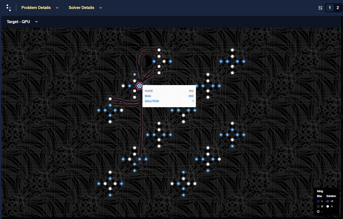
Fig. 71 A BQM with a single large-biased qubit that reduces the range of qubit biases available for the remaining linear biases.#
>>> import dimod
>>> import networkx as nx
>>> from dwave.system import DWaveSampler
>>> import dwave_networkx as dnx
>>> from dwave.preprocessing import FixVariablesComposite
...
>>> # Create a native problem with one outsized bias
>>> coords = dnx.pegasus_coordinates(16)
>>> qpu = DWaveSampler(solver={'topology__type': 'pegasus'})
>>> p16_working = dnx.pegasus_graph(16, node_list=qpu.nodelist, edge_list=qpu.edgelist)
>>> p12k44_nodes = [coords.nice_to_linear((t, y, x, u, k)) for (t, y, x, u, k) in list(coords.iter_linear_to_nice(p16_working.nodes)) if x in [2, 3] and y in [2, 3]]
>>> p12k44 = p16_working.subgraph(p12k44_nodes)
>>> bqm = dimod.generators.randint(p12k44, "SPIN")
>>> bqm.set_linear(list(bqm.linear.keys())[0], -100)
...
>>> # Submit with and without the outsized bias
>>> sampleset = qpu.sample(bqm, num_reads=1000)
>>> sampler_fixed = FixVariablesComposite(qpu)
>>> sampleset_fixed = sampler_fixed.sample(bqm, fixed_variables={bqm.variables[0]: 1}, num_reads=1000)
The two figures below show the energies of returned solutions:
Figure 72 is the BQM with the outsized bias.
Figure 73 is the (updated) BQM without the outsized bias.
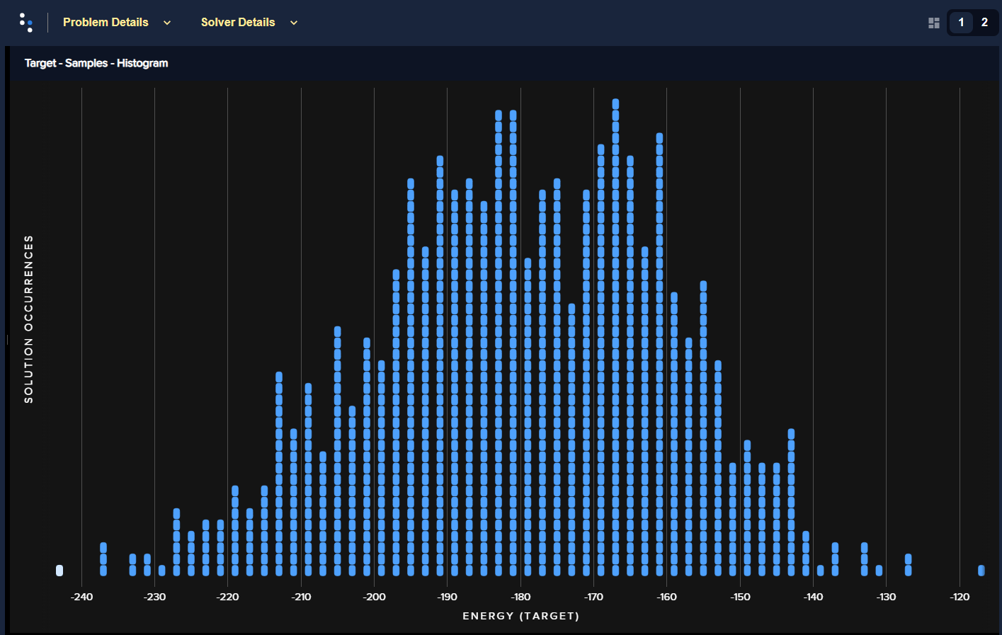
Fig. 72 Energies of returned solutions for the original BQM with the outsized bias.#
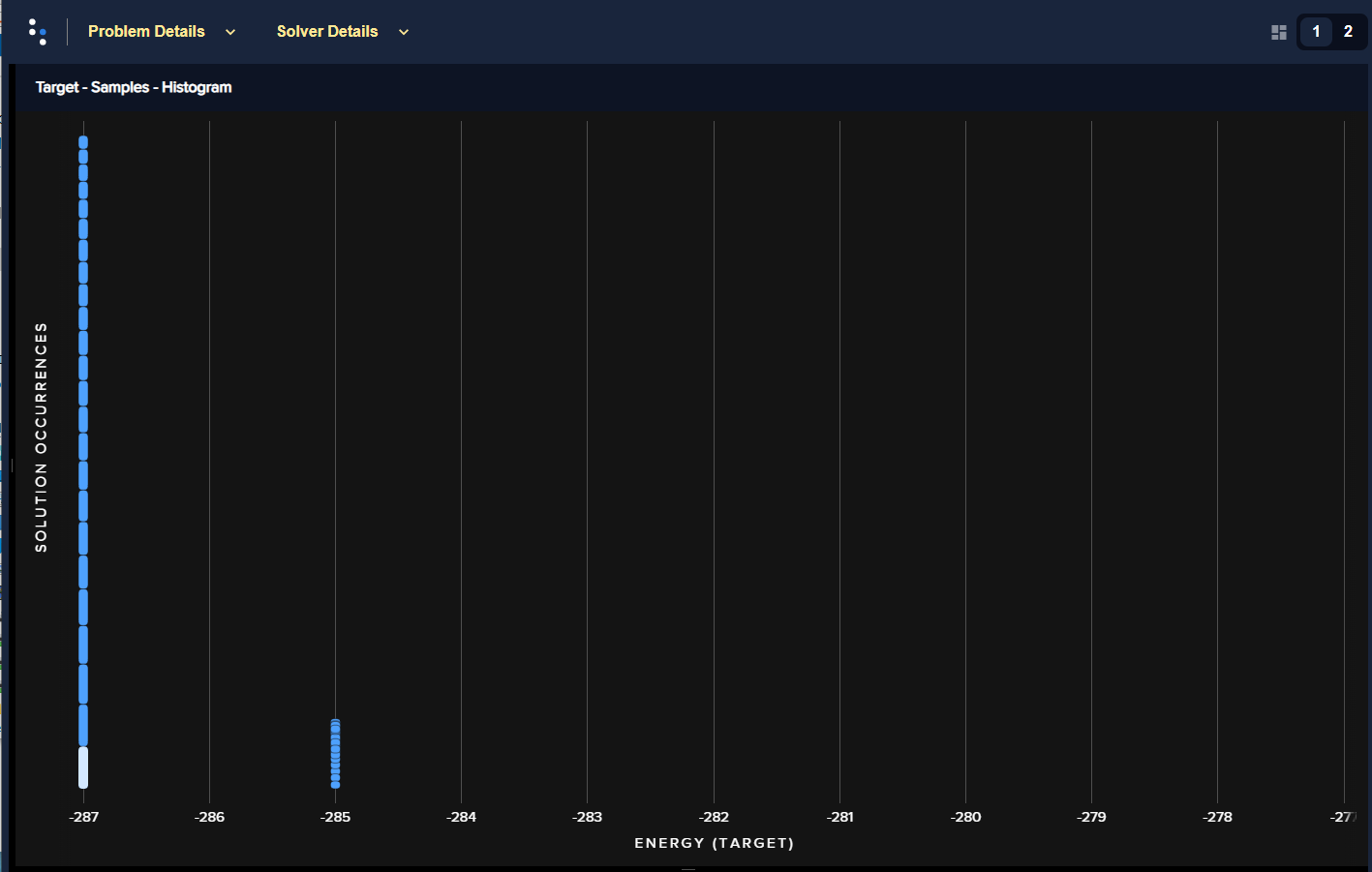
Fig. 73 Energies of returned solutions for the BQM with the variable that has an outsized bias fixed.#
When the original BQM is embedded on the QPU, the problem range is scaled by 25:
>>> print(min(bqm.linear.values())//min(qpu.properties["h_range"]))
25.0
The qubit biases of all but one variable and the coupler strengths are either 0
or 0.04; that is, over 99% of the qubit biases are in just 0.5% of the available
range of \(h\) values ([-4.0, 4.0] for the QPU on which this example
was run).
In a fixed BQM, most variables keep the original coefficient values except for variables connected to the fixed variable. For this execution of the example, two connected variables’ coefficients are changed to a value of 2 to account for the fixed variable.
>>> bqm.fix_variable(bqm.variables[0], 1)
>>> set(bqm.quadratic.values()) | set(bqm.linear.values())
{0.0, 1.0, 2.0}
>>> print(bqm.linear.max()/max(qpu.properties["h_range"]))
0.5
Annealing Schedule#
Some types of problems benefit from the introduction of a pause or a quench at some point in the anneal schedule. A pause dwells for some time at a particular anneal fraction; a quench abruptly terminates the anneal within a few hundred nanoseconds of the point specified.
This degree of control over the global annealing schedule also enables closer study the quantum annealing algorithm.
Pause and Quench#
A pause can be a useful diagnostic tool for instances with a small perturbative anticrossing. While pauses early or late in the anneal have no effect, a pause near the expected perturbative anticrossing produces a large increase in the ground-state success rate.
If a quench is fast compared to problem dynamics, then the distribution of states returned by the quench can differ significantly from that returned by the standard annealing schedule. The probability of obtaining ground state samples depends on when in the anneal the quench occurs, with later quenches more likely to obtain samples from the ground state.
Supply the scheduling points using the anneal_schedule solver parameter.
Reverse Anneal#
Reverse annealing enables the use of quantum annealing as a component in local search algorithms to refine classical states. Examples of using this feature include Quantum Boltzmann sampling, tunneling rate measurements, and relaxation rate measurements.
Examples#
Figure 74 shows embedded in an Advantage QPU a 16-qubit system, which was studied in a nature article. It has an energy gap of 4 between the classical ground state and excited states.
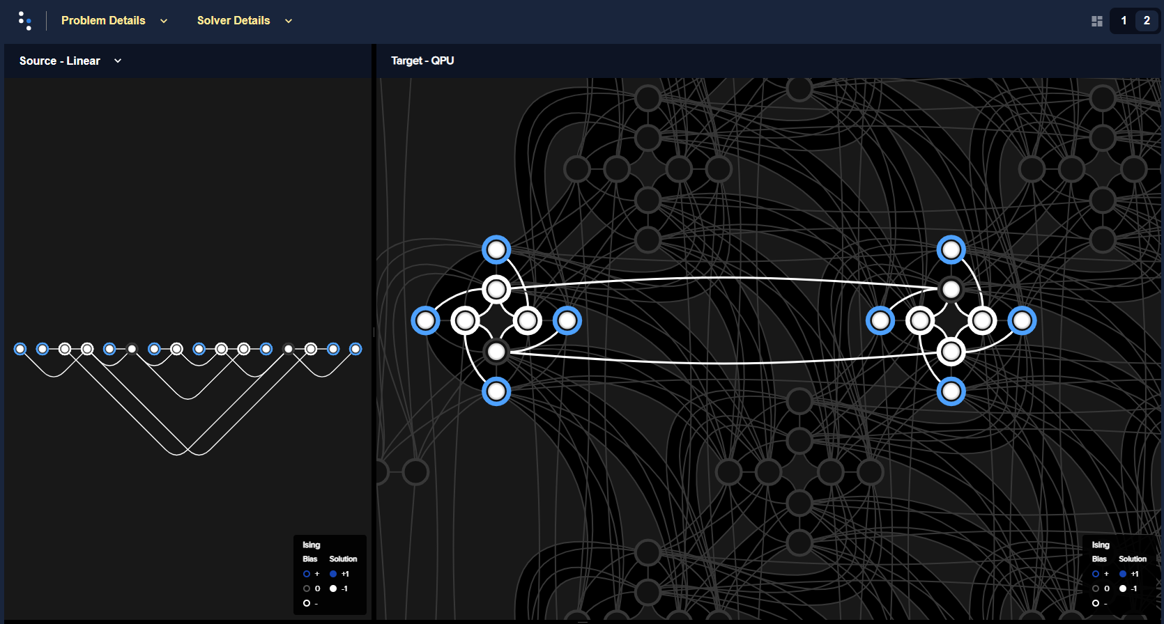
Fig. 74 A 16-qubit system with an energy gap of 4 between the classical ground state and excited states embedded in an Advantage QPU.#
The following code shows how varying the anneal schedule can increase the probability of finding ground states. (Results can vary significantly between executions.) First, the problem is embedded onto a QPU such that each problem qubit is represented by a single qubit[1] on the QPU.
>>> import numpy as np
>>> import dwave_networkx as dnx
>>> from dwave.system import DWaveSampler, FixedEmbeddingComposite
>>> from minorminer import find_embedding
...
>>> # Configure the problem structure
>>> h = {0: 1.0, 1: -1.0, 2: -1.0, 3: 1.0, 4: 1.0, 5: -1.0, 6: 0.0, 7: 1.0,
...      8: 1.0, 9: -1.0, 10: -1.0, 11: 1.0, 12: 1.0, 13: 0.0, 14: -1.0, 15: 1.0}
>>> J = {(9, 13): -1, (2, 6): -1, (8, 13): -1, (9, 14): -1, (9, 15): -1,
...      (10, 13): -1, (5, 13): -1, (10, 12): -1, (1, 5): -1, (10, 14): -1,
...      (0, 5): -1, (1, 6): -1, (3, 6): -1, (1, 7): -1, (11, 14): -1,
...      (2, 5): -1, (2, 4): -1, (6, 14): -1}
...
>>> # Find a Pegasus embedding
>>> qpu_pegasus = DWaveSampler(solver={'topology__type': 'pegasus'})
>>> embedding = find_embedding(J.keys(), qpu_pegasus.edgelist)
>>> max(len(val) for val in embedding.values()) == 1
True
>>> # Set up the sampler
>>> reads = 1000
>>> sampler = FixedEmbeddingComposite(qpu_pegasus, embedding)
Print the percentage of ground states for a 100 \(\mu s\) anneal:
>>> sampleset = sampler.sample_ising(h, J, num_reads=reads, answer_mode='raw',
...                                  annealing_time=100)
>>> counts = np.unique(sampleset.record.energy.reshape(reads,1), axis=0,
...                    return_counts=True)[1]
>>> print("{}% of samples were best energy {}.".format(100*counts[0]/sum(counts),
...       sampleset.first.energy))
6.8% of samples were best energy -20.0.
Print the percentage of ground states for an anneal with a 100 \(\mu s\) pause:
>>> anneal_schedule=[[0.0, 0.0], [40.0, 0.4], [140.0, 0.4], [142, 1.0]]
>>> sampleset = sampler.sample_ising(h, J, num_reads=reads, answer_mode='raw',
...                                  anneal_schedule=anneal_schedule)
>>> counts = np.unique(sampleset.record.energy.reshape(reads,1), axis=0,
...                    return_counts=True)[1]
>>> print("{}% of samples were best energy {}.".format(100*counts[0]/sum(counts),
...       sampleset.first.energy))
28.7% of samples were best energy -20.0.
Print the percentage of ground states for a reverse anneal (of almost 100 \(\mu s\)):
>>> reverse_schedule = [[0.0, 1.0], [5, 0.55], [99, 0.55], [100, 1.0]]
>>> initial = dict(zip(sampleset.variables, sampleset.record[int(reads/2)].sample))
>>> reverse_anneal_params = dict(anneal_schedule=reverse_schedule,
...                              initial_state=initial,
...                              reinitialize_state=True)
>>> sampleset = sampler.sample_ising(h, J, num_reads=reads, answer_mode='raw',
...                                  **reverse_anneal_params)
>>> counts = np.unique(sampleset.record.energy.reshape(reads,1), axis=0,
...                    return_counts=True)[1]
>>> print("{}% of samples were best energy {}.".format(100*counts[0]/sum(counts),
...       sampleset.first.energy))
99.7%% of samples were best energy -20.0.
Further Information#
Jupyter Notebooks Anneal Schedule and Reverse Anneal demonstrate these features.
[Dic2013] discusses the anticrossing example.
[Dwave5] is a white paper on reverse annealing.
[Izq2022] shows the efficacy of mid-anneal pauses.
The QPU Solver Datasheet guide describes varying the anneal schedule.
Anneal Offsets#
Anneal offsets may improve results for problems in which the qubits have irregular dynamics for some easily determined reason; for example, if a qubit’s final value does not affect the energy of the classical state, you can advance it (with a positive offset) to reduce quantum bias in the system.
Anneal offsets can also be useful in embedded problems with varying chain length: longer chains may freeze out earlier than shorter ones, which means that at an intermediate point in the anneal, some variables act as fixed constants while others remain undecided. If, however, you advance the anneal of the qubits in the shorter chains, they freeze out earlier than they otherwise would. The correct offset will synchronize the annealing trajectory of the shorter chains with that of the longer ones.
If you decide that offsetting anneal paths might improve results for a problem, your next task is to determine the optimal value for the qubits you want to offset. As a general rule, if a qubit is expected to be subject to a strong effective field relative to other qubits, delay its anneal with a negative offset. The ideal offset magnitudes are likely to be the subject of trial and error, but expect that the appropriate offsets for two different qubits in the same problem to be within 0.2 normalized offset units of each other.
Supply the array of offsets for the qubits in the system using the anneal_offsets solver parameter with a length equal to the num_qubits property.
Example: 3-Qubit System#
This example is a 3-qubit looks at a system that has a ground state, \(1, 1, 1\), separated from its two closest excited states, \(-1, -1, -1\) and \(-1, -1, 1\), by a small energy gap compared to its remaining excited states. These two first excited states have the same energy and differ by a single flip of qubit 2; consequently, the superposition of these two states is dominant early in the anneal. Figure 76 shows the problem and a possible embedding in one particular Advantage QPU.
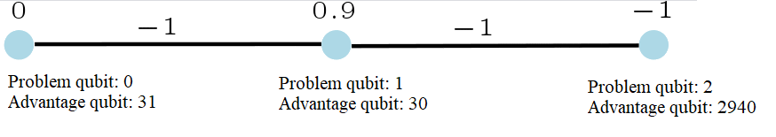
Fig. 76 A three-qubit system with a small energy gap between the ground state and first two excited states.#
dimod‘s
ExactSolver shows the energies of the ground
state, first two excited states, and remaining states:
>>> from dimod import ExactSolver
>>> h = {0: 0, 1: 0.9, 2: -1}
>>> J = {(0, 1): -1, (1, 2): -1}
>>> print(ExactSolver().sample_ising(h, J))
   0  1  2 energy num_oc.
5 +1 +1 +1   -2.1       1
0 -1 -1 -1   -1.9       1
7 -1 -1 +1   -1.9       1
4 -1 +1 +1   -0.1       1
1 +1 -1 -1    0.1       1
6 +1 -1 +1    0.1       1
2 +1 +1 -1    1.9       1
3 -1 +1 -1    3.9       1
['SPIN', 8 rows, 8 samples, 3 variables]
The D-Wave system used for this example is an Advantage that has couplers between active qubits 30, 31, and 2940. Select a suitable embedding for the QPU you run examples on.
>>> from dwave.system import FixedEmbeddingComposite, DWaveSampler
>>> qpu = DWaveSampler()
>>> embedding = {0: [31], 1: [30], 2: [2940]}
>>> sampler = FixedEmbeddingComposite(qpu, embedding)
>>> print(qpu.properties['anneal_offset_ranges'][2940])
[-0.7012257815714587, 0.6717794151250857]
For the default anneal offset of qubit 2, this particular run of 1000 samples, successfully returned the problem’s ground state about one third of the time, and likewise each of the two first excited states a third of the time:
>>> sampleset = sampler.sample_ising(h, J, num_reads=1000)
>>> print(sampleset)
   0  1  2 energy num_oc. chain_.
0 +1 +1 +1   -2.1     386     0.0
1 -1 -1 +1   -1.9     276     0.0
2 -1 -1 -1   -1.9     338     0.0
['SPIN', 3 rows, 1000 samples, 3 variables]
Applying a positive offset to qubit 2 causes it to freeze a bit earlier in the anneal than qubits 0 and 1. Consequently, the superposition of the two lowest excited states, \(-1, -1, -1\) and \(-1, -1, 1\), no longer dominates, and the ground state is found much more frequently.
>>> offset = [0]*qpu.properties['num_qubits']
>>> offset[2940]=0.2
>>> sampleset = sampler.sample_ising(h, J, num_reads=1000, anneal_offsets=offset)
>>> print(sampleset)
   0  1  2 energy num_oc. chain_.
0 +1 +1 +1   -2.1     979     0.0
1 -1 -1 +1   -1.9       7     0.0
2 -1 -1 -1   -1.9      13     0.0
3 -1 +1 +1   -0.1       1     0.0
['SPIN', 4 rows, 1000 samples, 3 variables]
Example: 16-Qubit System#
The example problem of the Annealing Schedule section improved solutions for a 16-qubit system, shown in Figure 74 embedded in an Advantage QPU, which was studied in a nature article, and has an energy gap of 4 between the classical ground state and excited states. The eight “outer” qubits, which are coupled to only one other qubit, enable single flips that produce dominant superpositions of excited states in the anneal (these are small-gap anticrossings), reducing the likelihood of finding the ground state.
First, the problem is embedded onto a QPU such that each problem qubit is represented by a single qubit on the QPU. As explained in the Annealing Schedule section, on most executions, Ocean software’s minorminer finds an embedding with all chains of length 1. However, a typical embedding looks like that of Figure 75. The following code finds a more visually intuitive embedding such as shown in Figure 74 above.
>>> import itertools
>>> import numpy as np
>>> import dwave_networkx as dnx
>>> from dwave.system import DWaveSampler, FixedEmbeddingComposite
>>> from minorminer import find_embedding
...
>>> # Configure the problem structure
>>> h = {0: 1.0, 1: -1.0, 2: -1.0, 3: 1.0, 4: 1.0, 5: -1.0, 6: 0.0, 7: 1.0,
...      8: 1.0, 9: -1.0, 10: -1.0, 11: 1.0, 12: 1.0, 13: 0.0, 14: -1.0, 15: 1.0}
>>> J = {(9, 13): -1, (2, 6): -1, (8, 13): -1, (9, 14): -1, (9, 15): -1,
...      (10, 13): -1, (5, 13): -1, (10, 12): -1, (1, 5): -1, (10, 14): -1,
...      (0, 5): -1, (1, 6): -1, (3, 6): -1, (1, 7): -1, (11, 14): -1,
...      (2, 5): -1, (2, 4): -1, (6, 14): -1}
...
>>> # Find an embedding with a single QPU qubit representing each problem qubit
>>> qpu_pegasus = DWaveSampler(solver={'topology__type': 'pegasus'})
>>> coords = dnx.pegasus_coordinates(16)
>>> try:
...     for x, y, t in itertools.product(range(15), range(16), range(3)):
...         nodes = {s: [coords.nice_to_linear((t, y, x + s//8, 1 if s%8//4 else 0 , s%4))]
...                  for s in h.keys()}
...         try:
...             embedding = find_embedding(J.keys(), qpu_pegasus.edgelist, restrict_chains=nodes)
...         except Exception:
...             pass
...         else:
...             break
>>> # Set up the sampler
>>> reads = 1000
>>> sampler = FixedEmbeddingComposite(qpu_pegasus, embedding)
Figure 77 shows the 16-qubit system embedded in an Advantage QPU.
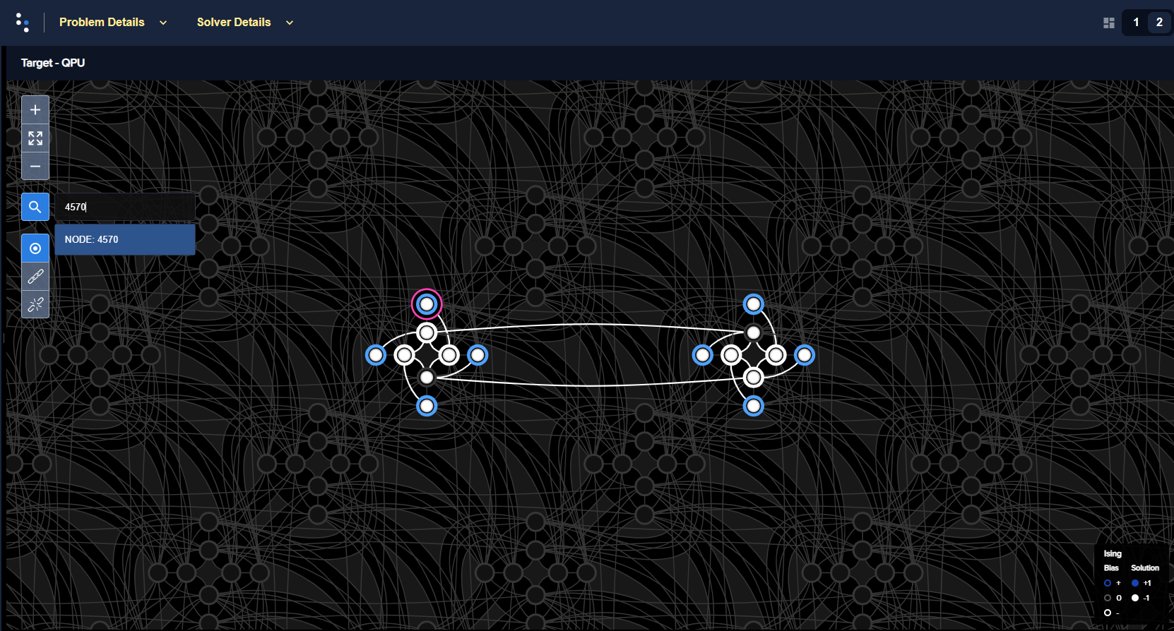
Fig. 77 A 16-qubit system with an energy gap of 4 between the classical ground state and excited states embedded in an Advantage QPU. One of the eight “outer” qubits, problem qubit 4, which is embedded here to QPU qubit 4570, is highlighted.#
The following code samples 1000 times, with an anneal time of 100 \(\mu s\) and no annealing offsets, and prints the percentage of ground states found.
>>> offset = [0]*qpu_pegasus.properties['num_qubits']
>>> sampleset = sampler.sample_ising(h, J, num_reads=reads, answer_mode='raw',
...                                  annealing_time=100,
...                                  anneal_offsets=offset)
>>> counts = np.unique(sampleset.record.energy.reshape(reads,1), axis=0,
...                    return_counts=True)[1]
>>> print("{}% of samples were best energy {}.".format(100*counts[0]/sum(counts),
...       sampleset.first.energy))
8.2% of samples were best energy -20.0.
The minimum range for a positive anneal offset for any of the eight “outer” qubits of this example’s particular embedding can be found as below:
>>> ao_range = qpu_pegasus.properties["anneal_offset_ranges"]
>>> ao_step = qpu_pegasus.properties["anneal_offset_step"]
>>> outer8 = [4570, 1913, 4615, 1868, 4571, 2093, 4616, 2048]
>>> print(min([ao_range[outer][1] / abs(ao_step) for outer in outer8]))
3533.0651831083146
The following code samples 1000 times, with an anneal time of 100 \(\mu s\) and annealing offsets set for the eight “outer” qubits, and prints the percentage of ground states found.
>>> for outer in outer8:
...     offset[outer] = 300*abs(ao_step)
>>> sampleset = sampler.sample_ising(h, J, num_reads=reads, answer_mode='raw',
...                                  annealing_time=100,
...                                  anneal_offsets=offset)
>>> counts = np.unique(sampleset.record.energy.reshape(reads,1), axis=0,
...                    return_counts=True)[1]
>>> print("{}% of samples were best energy {}.".format(100*counts[0]/sum(counts),
...       sampleset.first.energy))
99.8% of samples were best energy -20.0.
Further Information#
QPU Solver Datasheet describes anneal offsets.
[Dwave3] describes boosting factoring using anneal oofsets.
[Kin2016] discusses the use of anneal offsets.
[Lan2017] shows the use of anneal offsets on several problems.
[Tin2018] systematically applies anneal offsets to SAT problems.
Emulate Linear Biases with Flux-Bias Offsets#
It is sometimes useful to represent linear coefficients on a problem’s variables without setting biases on the corresponding qubits; for example, when running the fast-anneal protocol. This protocol does not allow non-zero values for h or diagonal elements of Q, so to represent part of a problem modeled, for example, as \(a_{1,2}x_1x_2 + a_2x_2\) one needs to bias the qubit or qubits representing \(x_2\) without applying a bias \(h_2=a_2.\)
You can use flux-bias offsets for this purpose. Locate an unused neighboring qubit that can be coupled to the problem qubit, apply to this ancillary qubit a flux-bias offset of magnitude greater than \(JM_{\rm AFM} I_p / \Phi_0\) (see equation (2) in the QPU Solver Datasheet guide), and set the coupling strength between the problem and ancillary qubits equal to the needed linear bias.
Figure 78 shows the ratio of spin states \(-1\) and \(+1\) for a qubit, \(q1\), annealed 1000 times for each value, in range \([-1.0, 1.0]\), of these two methods of biasing its outcome:
Qubit \(q1\) is biased by \(h_1\) (the standard way of biasing a qubit to represent the linear coefficient of a problem variable).
Qubit \(q1\) is coupled to ancillary qubit \(q_2\) by \(J_{1,2}\). A flux-bias offset of large magnitude is applied to ancillary qubit \(q_2\).
As is seen, directly biasing the problem qubit, \(q_1\), with linear bias \(h_1\) is equivalent to coupling it to flux-biased ancillary qubit \(q_2\) with a coupling strength of \(J_{1,2}\), as long as the magnitude of the flux-bias offset is high enough.
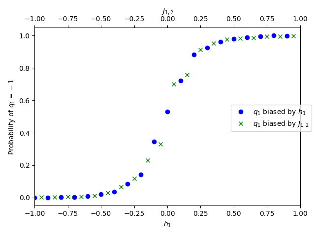
Fig. 78 Ratio of states for a qubit biased with \(h_1\) or coupled with \(J_{1,2}\) to a second qubit on which a high flux-bias offset is applied.#
The following code snippet provides a single-point demonstration. Scan across h_1
and J_12 to reproduce the plots of Figure 78 above.
>>> import numpy as np
>>> from dwave.system import DWaveSampler
...
>>> qpu = DWaveSampler()
>>> q1, q2 = qpu.edgelist[0]
...
>>> h_1 = 0.25
>>> J_12 = 0.25
...
>>> fb = [0]*qpu.properties['num_qubits']
>>> sampleset1 = qpu.sample_ising({q1: h_1, q2: 0}, {(q1, q2): 0}, num_reads=1000, auto_scale=False,
...                              answer_mode="raw", flux_biases=fb)
>>> fb[q2] = 0.001
>>> sampleset2 = qpu.sample_ising({q1: 0, q2: 0}, {(q1, q2): J_12}, num_reads=1000,
...                              auto_scale=False, answer_mode="raw", flux_biases=fb)
>>> sample1 = sampleset1.record.sample
>>> sample2 = sampleset2.record.sample
>>> print(np.count_nonzero(sample1[:,0]==-1)/sample1.shape[0])
0.855
>>> print(np.count_nonzero(sample2[:,0]==-1)/sample2.shape[0])
0.858
Energy Gap#
There are strategies for increasing the gap between ground and excited states during the anneal. For example, different choices of constraints when reformulating a CSP as a QUBO affect the gap.
Consider also the differences between maximizing the gap versus creating a uniform gap.
Example#
This example formulates a 3-bit parity check[2] as an Ising model in two ways, the first with an energy gap of 1 and the second with an energy gap of 2.
Penalty model 1 is formulated as,
with one auxiliary variable, \(a\), and an energy gap of 1. The following code samples it on an Advantage QPU:
>>> from dwave.system import DWaveSampler, EmbeddingComposite
>>> sampler = EmbeddingComposite(DWaveSampler(solver={'topology__type': 'pegasus'}))
>>> h = {'s1': 0.5, 's2': 0.5, 's3': 0.5, 'a': -1}
>>> J = {('s1', 's2'): 0.5, ('s1', 's3'): 0.5, ('s2', 's3'): 0.5,
...      ('s1', 'a'): -1, ('s2', 'a'): -1, ('s3', 'a'): -1}
>>> sampleset = sampler.sample_ising(h, J, num_reads=1000)
>>> print(sampleset)
    a s1 s2 s3 energy num_oc. chain_.
0  +1 -1 +1 +1   -2.0     209     0.0
1  +1 +1 +1 -1   -2.0     244     0.0
2  -1 -1 -1 -1   -2.0     265     0.0
3  +1 +1 -1 +1   -2.0     271     0.0
4  -1 +1 -1 -1   -1.0       1     0.0
5  -1 -1 -1 +1   -1.0       1     0.0
6  -1 -1 +1 -1   -1.0       1     0.0
7  +1 +1 +1 +1   -1.0       1     0.0
8  +1 -1 +1 -1   -1.0       2     0.0
9  +1 -1 -1 +1   -1.0       2     0.0
10 +1 +1 -1 -1   -1.0       3     0.0
['SPIN', 11 rows, 1000 samples, 4 variables]
Penalty model 2 is formulated as,
with three auxiliary variables, \(a_1, a_2, a_3\), and an energy gap of 2. The following code samples it on the same Advantage QPU as the previous code:
>>> h = {'a1': -1, 'a2': 1, 'a3': -1}
>>> J = {('s1', 'a1'): 1, ('s1', 'a2'): 1, ('s1', 'a3'): 1,
...      ('s2', 'a1'): -1, ('s2', 'a2'): 1, ('s2', 'a3'): 1,
...      ('s3', 'a1'): 1, ('s3', 'a2'): 1, ('s3', 'a3'): -1}
>>> sampleset = sampler.sample_ising(h, J, num_reads=1000)
>>> print(sampleset)
  a1 a2 a3 s1 s2 s3 energy num_oc. chain_.
0 -1 -1 +1 +1 -1 +1   -6.0     302     0.0
1 +1 -1 -1 +1 +1 -1   -6.0     181     0.0
2 +1 +1 +1 -1 -1 -1   -6.0     278     0.0
3 +1 -1 +1 -1 +1 +1   -6.0     236     0.0
4 +1 +1 +1 -1 +1 -1   -4.0       1     0.0
5 -1 +1 +1 -1 -1 +1   -4.0       1     0.0
6 +1 +1 +1 -1 +1 +1   -2.0       1     0.0
['SPIN', 7 rows, 1000 samples, 6 variables]
For this simple example, both formulations produce a high percentage of ground states (states where the number of spin-up values for variables \(s_1, s_2, s_3\) is even). Had this been part of a more complex problem, you might have needed to weigh the benefit of a larger energy gap against other considerations, such as a larger number of ancillary variables.
Further Information#
Neighbor Interactions#
The dynamic range of \(h\) and \(J\) values may be limited by ICE. Instead of finding low-energy states to an optimization problem defined by \(h\) and \(J\), the QPU solves a slightly altered problem that can be modeled as
where the ICE errors \(\delta h_i\) and \(\delta J_{i,j}\) depend on \(h_i\) and on the values of all incident couplers \(J_{i,j}\) and neighbors \(h_j\), as well as their incident couplers \(J_{j,k}\) and next neighbors \(h_k\). For example, if a given problem is specified by \((h_1 = 1 , h_2 = 1, J_{1,2} = -1)\), the QPU might actually solve the problem \((h_1 = 1.01, h_2 = 0.99, J_{1,2} = -1.01)\).
Changing a single parameter in the problem might change all three error terms, altering the problem in different ways.
Further Information
[Har2010] discusses how applied \(h\) bias leaks from spin \(i\) to its neighboring spins.