Error Sources for Problem Representation

The dynamic range of \(h\) and \(J\) values may be limited by integrated control errors (ICE). The term ICE refers collectively to these sources of infidelity in problem representation. This chapter provides an overview of ICE, describes the main sources that contribute to it, and provides guidance on measuring its effects.

Note

Data given in this chapter are representative of D-Wave systems.

Overview of ICE

Although \(h\) and \(J\) may be specified as double-precision floats, some loss of fidelity occurs in implementing these values in the D-Wave QPU. This fidelity loss may affect performance for some types of problems.

Specifically, instead of finding low-energy states to an optimization problem defined by \(h\) and \(J\) as in equation (1), the QPU solves a slightly altered problem that can be modeled as

\begin{equation} E^{\delta}_{ising} ({\bf s}) = \sum_{i=1}^N (h_i + \delta h_i ) s_i + \sum_{i=1}^N \sum_{j=i+1}^{N} (J_{i,j} + \delta J_{i,j} ) s_i s_j, \end{equation}

where \(\delta h_i\) and \(\delta J_{i,j}\) characterize the errors in parameters \(h_i\) and \(J_{i,j}\), respectively.[1]

[1]

Because \(\delta h\) and \(\delta J\) are summed over \(N\), fidelity limitations tend to have a greater effect on performance for full-QPU sized problems, for a given dynamic range and distribution of \(h\) and \(J\).

The error \(\delta h_i\) depends on \(h_i\) and on the values of all incident couplers \(J_{i,j}\) and neighbors \(h_j\), as well as their incident couplers \(J_{j,k}\) and next neighbors \(h_k\). That is, if spin \(i\) is connected to spin \(j\), and spin \(j\) is connected to spin \(k\) in the topological graph, then \(\delta h_i\) may depend, to varying extents, on \(h_i, h_j, h_k\), \(J_{i,j}\), and \(J_{j,k}\). This dependency holds when the relevant qubits and couplings are present in the graph, irrespective of whether they are set to nonzero values. Similarly, \(\delta J_{i,j}\) depends on spins and couplings in the local neighborhood of \(J_{i,j}\). For example, if a given problem is specified by \((h_1 = 1 , h_2 = 1, J_{1,2} = -1)\), the QPU might actually solve the problem \((h_1 = 1.01, h_2 = 0.99, J_{1,2} = -1.01)\). Changing just a single parameter in the problem could change all three error terms, altering the problem in different ways.

The probability distribution of \(\delta h\) and \(\delta J\) is an ensemble across a set of problem settings \(h\) and \(J\) and across all \(i\) and \(i,j\) pairs. The \(\delta h\) and \(\delta J\) values are Gaussian-distributed with mean \(\mu\) and standard deviation \(\sigma\) that vary with anneal fraction \(s\) during the anneal.[2] The QPU control system is calibrated so that there is typically a value of \(s\) for which \(\mu\) is zero. This point is chosen to be somewhere between the single qubit freezeout point described in the Freezeout Points section (later in the anneal), and at the quantum critical point of a one-dimensional Ising chain (earlier in the anneal). Distributions with nonzero \(\mu\) for some values of \(s\) are considered to be due to systematic errors discussed later in this chapter. Thus, the expected deviations of \(h\) and \(J\) during operation are the sum of a systematic contribution \(\mu\) and a random component with standard deviation \(\sigma.\)

[2]

Assumed for simplicity; distributions seen in actual results are close to this.

Figure 94 and Figure 95 show example measurements of \(\delta h\) and \(\delta J\) distributions at different fractional times \(s\). See the Using Two-Spin Systems to Measure ICE section for a description of the measurement method.

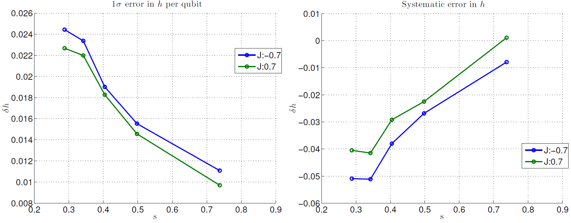
Fig. 94 \(\delta h\) distributions estimated from best-fit parameters to a thermal model. The left plot shows the standard deviation of the distribution and the right plot shows the mean. Data were taken for logical qubits between size 1 (larger \(s\)) and size 5 (smaller \(s\)) to get an estimate of \(\delta h\) over a range of \(s\). Data shown are representative of D-Wave 2X systems.

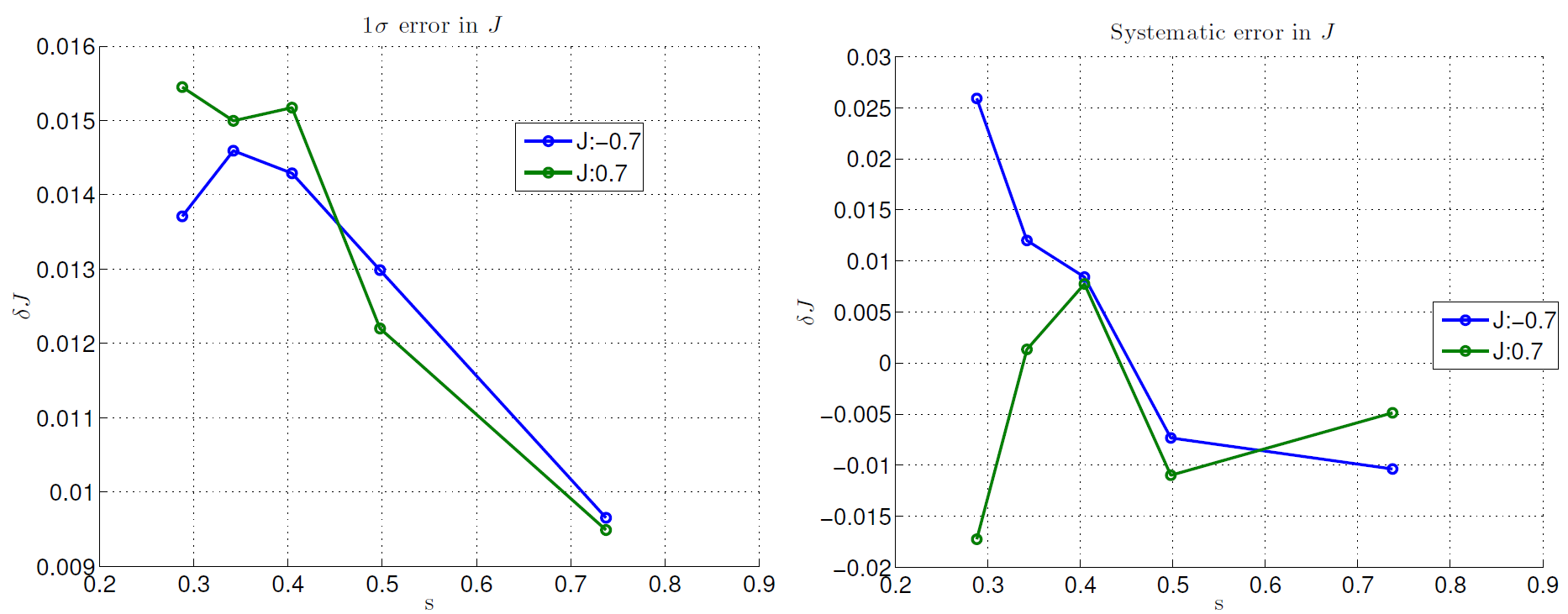
Fig. 95 \(\delta J\) distributions estimated from best-fit parameters to a thermal model. The left plot shows the standard deviation of the distribution and the right plot shows the mean. Data were taken for logical qubits between size 1 (larger \(s\)) and size 5 (smaller \(s\)) to get an estimate of \(\delta J\) over a range of \(s\). Data shown are representative of D-Wave 2X systems.

Sources of ICE

The Ising spins on the D-Wave QPU are intrinsically analog, controlled through spatially local magnetic fields. The controls are a combination of the output of on-QPU DACs and other analog signals shared among groups of spins. A calibration procedure, conducted when the QPU first comes online, determines the mapping between Ising problem specifications \(h\) and \(J\), and the control values used during annealing.

QPU calibration is a significant part of the time required to install a D-Wave system at a site. It involves a series of measurements of the QPU and the refrigerator to obtain data used to build models that achieve the desired Ising spin Hamiltonian.

These models identify several factors that contribute to distortions of \(h\) and \(J\) due to ICE. Understanding these factors, and how to compensate for them, can guide your choices in \(h\) and \(J\) when you specify a problem. Listed below are the dominant sources of ICE. The subsections that follow give additional details.

• Background Susceptibility (ICE1)

  The on-QPU rf-SQUID qubits behave weakly as couplers, which leads to effective next-nearest-neighbor (NNN) \(J\) interactions and a leakage of applied \(h\) biases from a qubit to its neighbors.

• Flux Noise of the Qubits (ICE2)

  The qubits experience low-frequency \(1/f\)-like flux noise. This noise contributes an error that varies in time (that is, between runs on the QPU), and also varies with \(s\).

• DAC Quantization (ICE3)

  The on-QPU DACs that provide the specified \(h\) and \(J\) values have a finite quantization step size.

• I/O System Effects (ICE4)

  The ratio of \(h/J\) may differ slightly for different annealing parameters such as \(t_f\).

• Distribution of h Scale Across Qubits (ICE5)

  Qubits cannot be made perfectly identical. As a result, individual spins may have slightly different magnitudes (persistent currents) and tunneling energies. These differences also vary with anneal fraction \(s\).

Background Susceptibility

During the annealing process, every Ising spin has a coupler-like effect on its neighbors (that is, the spins to which it is connected by couplings) that is not captured by the problem Hamiltonian. This effect takes two main forms:

• Spin \(i\) induces next-nearest neighbor (NNN) couplings between pairs of its neighboring spins.

• The applied \(h\) bias leaks from spin \(i\) to its neighboring spins.[3]

[3]

A more detailed description of how this arises from rf-SQUID qubits is in [Har2010].

The strength of this background susceptibility effect is characterized by a parameter \(\chi\).[4]

[4]

Use of the \(\chi\) symbol is consistent with the usage in physics of \(\chi\) to characterize the susceptibility of a magnetic system. This document uses a normalized \(\chi = M_{\rm AFM} \chi_q\), where \(M_{\rm AFM}\) is the maximum available antiferromagnetic mutual inductance, and \(\chi_q = \frac{dI_p}{d\Phi_q}\) is the physical qubit susceptibility.

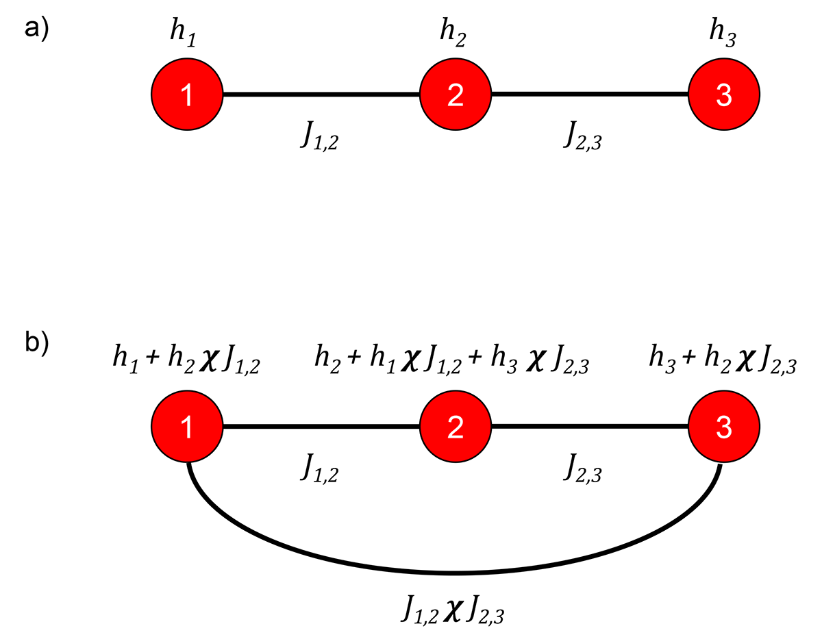
Fig. 96 a) Three-spin system to look at the effect of \(\chi\). Three spins, red circles, labeled \(1, 2, 3\) with local \(h\)-biases of \(h_1, h_2, h_3\), respectively, and couplings between neighboring spins denoted by lines of \(J_{1,2}\) between spin \(1\) and spin \(2\), and \(J_{2,3}\) between spin \(2\) and spin \(3\). b) The model for the system showing induced couplings and \(h\)-biases due to qubit susceptibility, \(\chi\).

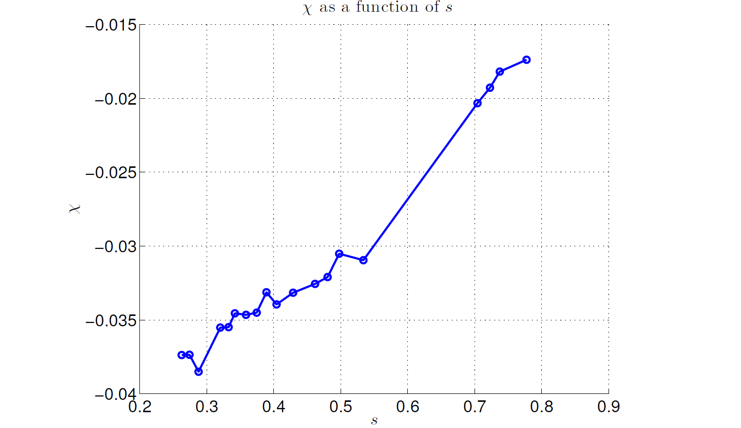
Fig. 97 \(\chi\) variation during the anneal. Data shown are representative of D-Wave 2X systems.

For example, consider the three-spin problem shown in Figure 96. This system is described by the Ising energy function

\begin{equation} E_{3} (\vc s) = + h_1 s_1 + h_2 s_2 + h_3 s_3 + J_{1,2} s_1 s_2 + J_{2,3} s_2 s_3. \end{equation}

The energy function solved by the QPU, however, has some extra terms:

\begin{equation} E^\delta_{\chi} (\vc s) = \underbrace{+ h_2 \chi J_{1,2} s_1 + h_1 \chi J_{1,2} s_2 + h_3 \chi J_{2,3} s_2 + h_2 \chi J_{2,3} s_3 }_\text{$h$ leakage} + \underbrace{ J_{1,2} \chi J_{2,3} s_1 s_3}_\text{NNN coupling}. \end{equation}

The NNN coupling occurs because spin 1 induces an interaction between spins 1 and 3 with magnitude \(J_{1,2} \chi J_{2,3}\). Similarly, \(h_2\) leaks onto spin 1, with magnitude \(h_2 \chi J_{1,2}\), and so on for the other terms.

Figure 97 shows how \(\chi\) typically varies with \(s\), from around -0.04 early in the anneal to near -0.015 late in the anneal, at which point single-spin dynamics freeze out.

Flux Noise of the Qubits

As another component of ICE, each \(h_i\) is subject to an independent (but time-dependent) error term that comes from the \(1/f\) flux noise of the qubits.[5] There are fluctuations in the flux noise that have lower frequency than the typical inverse annealing time, so problems solved in quick succession have correlated contributions from flux noise. By default, flux drift is automatically corrected every hour by the D-Wave system so that it is bounded and approximately Gaussian when averaged across all times; see the Drift Correction section for the procedure. You can disable this automatic correction by setting the flux_drift_compensation solver parameter to False. If you do so, apply flux-bias offsets manually; see the Flux-Bias Offsets section.

[5]

Couplers also have \(1/f\) flux noise, but this effect is insignificant compared to \(\delta h\) and \(\delta J\).

Because the physical source of noise is flux fluctuations on the qubits, the effective level of noise is larger earlier in the anneal when the persistent current in qubits is smaller, so that \(h\) is relatively smaller in physical flux units; see the Hardware: Coupled rf-SQUID Qubits section and the Characterizing the Effect of Flux Noise section for details.

The Fourier spectrum of the fluctuations of \(\delta h^2\) varies approximately as \(A^2/f^\alpha\), where \(f\) is frequency from 1 mHz to the highest-resolvable frequency, \(A\) is the amplitude of the fluctuations at \(f = 1\) Hz, and \(\alpha\) is the spectral tilt—or frequency dependence—of the fluctuations. Due to the flux drift compensation, the spectrum becomes flat and close to zero below 1 mHz. Integrating the noise from 1 mHz to 1 MHz (the relevant band of interest observable directly), the Gaussian contribution to \(\delta h\) is approximately 0.009 early in the anneal and less later in the anneal. Figure 98 shows typical data for a 64-qubit system.

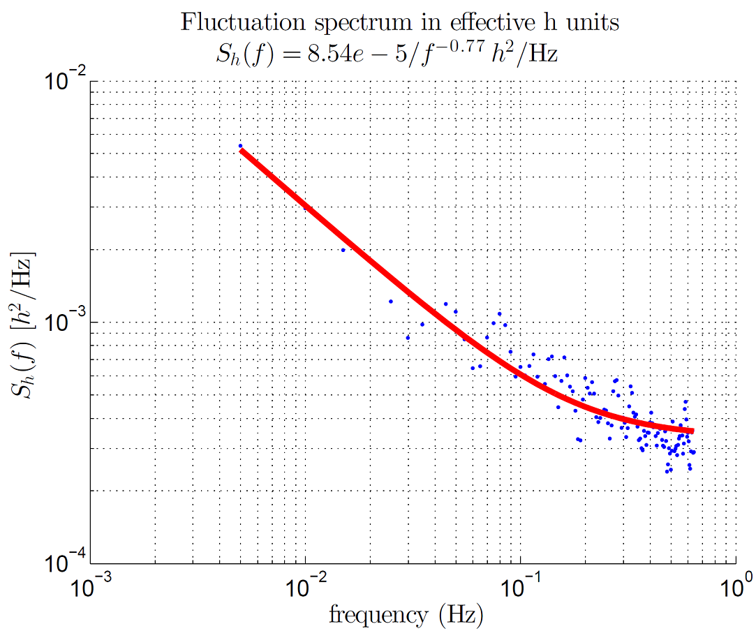
Fig. 98 Power spectral density of \(h\) fluctuations for a 64-qubit cluster. Data are taken by strongly coupling 64 qubits together and measuring the magnetization fluctuation of the system over time. The power spectral density of this signal, in effective \(h\) units, is plotted as a function of frequency. The solid line shows a best fit to the model \(A^2/f^{\alpha} + wn\), where \(wn\) is the statistical noise floor of the measurement technique and is not a measurement of any intrinsic broadband fluctuation of the qubit environment. See the Characterizing the Effect of Flux Noise section for more details. Data shown are representative of D-Wave 2X systems.

DAC Quantization

The on-QPU DACs that provide the user-specified \(h\) and \(J\) values have a finite quantization step size. That step size depends on the value of the \(h\) or \(J\) applied because the response to the DAC output is nonlinear.

This random error contribution is described by a uniform distribution centered at 0 and having errors \(\pm b\). Typical errors for \(h\) and \(J\) are shown in Figure 99. Note that these errors are smaller than other contributors to ICE.

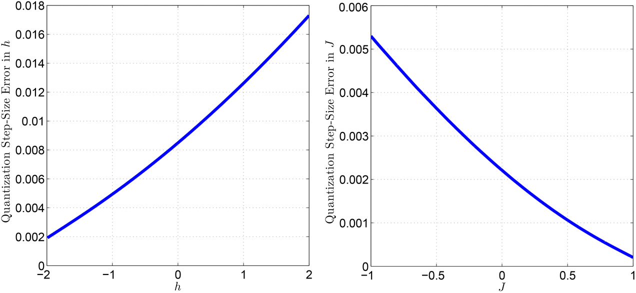
Fig. 99 Typical quantization step for the DAC controlling the \(h\) parameter (left) and \(J\) parameter (right). For example, \(h = 0.000\) may be off by as much as \(\pm 0.008\) when realized on the QPU. Over all qubits, you might find a worst-case qubit biased with \(h = 0.008\), and another worst-case qubit biased with \(h = -0.008\). Data shown are representative of D-Wave 2X systems.

I/O System Effects

Several time-dependent analog signals are applied to the QPU during the annealing process. Because the I/O system that delivers these signals has finite bandwidth,[6] the waveforms must be tuned for each anneal to minimize any potential distortion of the signals throughout the annealing process. As a result, the ratio of \(h/J\) may vary slightly with \(t_f\) and with scaled anneal fraction \(s\).

[6]

The anneal and h-controlling waveforms—\(\Phi_{\rm CCJJ}(s)\) and \(\Phi^x_i(s)\) terms, respectively, of equation (3) in the QPU Solver Datasheet guide—pass through low-pass filters with the following cutoff frequencies:

• For \(\Phi_{\rm CCJJ}(s)\): 30 MHz on both Advantage and Advantage2 systems

• For \(\Phi^x_i(s)\): 3 MHz for Advantage and 30 MHz for Advantage2

Distribution of \(h\) Scale Across Qubits

Assuming a fixed temperature of the system, and \(J=0\), the expected graph of the relationship between user-specified \(h\) and QPU-realized \(h\) has slope = 1, reflecting a constant mean offset \(\mu\) in the distribution of \(\delta h\). The measured slopes, however, are different for each spin, and are Gaussian-distributed.

This divergence results from small variations in the physical size of each qubit and from imperfections that arise when attempting to homogenize the macroscopic parameters—physical inductance \(L\), capacitance \(C\), and Josephson junction critical current \(I_c\)—across all physical qubits in the QPU.

Assuming a fixed temperature for the system, the ideal relationship, or slope, between qubit population and applied \(h\) is identical across an ensemble of devices. The distribution of measured slopes, however, is Gaussian-distributed with a standard deviation of approximately 1%, which contributes to \(\delta h\) and \(\delta J\). This distribution results from differences in the magnitude of each spin \(s_i\); see the Using Two-Spin Systems to Measure ICE section.

Measuring ICE

This section describes how to measure the effects of \(1/f\) noise as well as how to harness effective two-spin systems to measure the effects of ICE.

Measuring \(1/f\) Noise

A straightforward way to look at the \(1/f\) noise in the \(h\) parameter is to set all \(h\) and \(J\) values equal to 0 on the full QPU and observe how resulting qubit distributions drift over time in repeated tests. This approach identifies the effective \(1/f\) noise error on \(h\) when referenced to the single qubit freezeout point \(s^*_q\). To probe the \(1/f\) noise at earlier anneal times (and to amplify the error signal), create clusters of strongly coupled qubits and measure the time-dependent behavior of the net magnetization of system as described in the next section.

Using Two-Spin Systems to Measure ICE

You can use the results of problems defined on pairs of Ising spins scattered over the topological graph to help to characterize ICE effects.

Simple Two-Spin Systems

The simplest version of such problems has two Ising spins with biases \(h_1\) and \(h_2\) and a coupling between them of weight \(J\). The energy of this system is

(4)\[ E_{2spin}(\vc s) = +h_1 s_1 + h_2 s_2 + J s_1 s_2.\]

To measure ICE using simple two-spin systems, first find all independent edge sets of the available graph; that is, the sets of two-spin systems that can be manipulated independently. Simultaneously, for each set, ask the QPU to solve the independent two-spin problems at a variety of \(h_1\) and \(h_2\) settings near the phase boundaries indicated in Figure 100. Then fit the resulting data to a thermal model to estimate the deviations, \(\delta h\) and \(\delta J\), from equation (4) above using the correction terms of equation (5) below.

The two-spin phase diagram in Figure 100 characterizes the lowest energy state of the system as a function of \(h_1\) and \(h_2\) for given \(J\), here set to \(J=-0.5\). The dashed line delineates regions of the \(h_1\) and \(h_2\) space where resulting Ising spins are indicated by the up (\(s = 1\)) and down (\(s = -1\)) arrows. Applying a larger magnitude (more negative) \(J\) value increases ferromagnetic interactions, growing the regions of \(\downarrow \downarrow\) and \(\uparrow \uparrow\) while shrinking the regions of \(\downarrow \uparrow\) and \(\uparrow \downarrow\).

The ideal diagram may be compared to one obtained assuming the existence of background susceptibility errors. For this problem, the \(\chi\) correction terms are

(5)\[ E^\delta_{2spin} (\vc s) = +h_2 \chi J s_1 + h_1 \chi J s_2.\]

The \(h\)-leakage effects are shown in Figure 100: the blue lines denote the boundaries of the different spin ordering regions for the case where \(\chi = -0.05\), versus the ideal case shown by the dashed lines. (The two-spin system does not have NNN effects.)

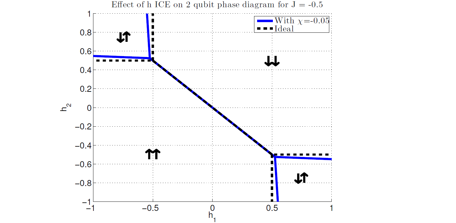
Fig. 100 Two-qubit (two Ising spin) phase diagram for \(J = -0.5\). The dashed lines show the locations of the expected phase boundaries between the four possible states of the system under the assumption of ideal Ising spin behavior. The solid lines show the locations of the phase boundaries for \(\chi = -0.05.\) To estimate the Ising spin parameters without systematic bias, \(\chi\) must be included in any model of the physical system. Data shown are representative of D-Wave 2X systems.

Given the form of the \(h\)-leakage terms, applying small adjustments to the \(h\) biases on the original problem can compensate somewhat for this error. However, \(\chi\) varies during the anneal (see Figure 97), and this correction corresponds to one specific point during the anneal. The single qubit freezeout point for typical anneal times occurs when \(s \approx 0.8\) and \(A(s)\) is around 100 MHz (see Figure 79). This is the last point in the anneal where any meaningful spin-flip dynamics occur; at that point \(\chi\) is approximately -0.015, so that value can, in principle, compensate for \(h\)-leakage. A better approach, however, is to choose \(\chi\) to correspond to a point earlier in the anneal—at or before the crossing point of \(A(s)\) and \(B(s)\). This is the localization point of a one-dimensional chain of spins.

Effective Two-Spin Systems For Larger Problems

Similar measurements may be repeated for larger problems made up of logical spins formed by strongly coupled groups of spins with strong intracluster coupling weights \(J_{cluster}\). Pairs of clusters are connected by the intercluster coupling weight \(J\), and the \(h_1\) and \(h_2\) weights are assigned to all spins in each cluster. These clusters freeze out at different anneal times depending on the number of spins and on coupling strengths \(J\) and \(J_{cluster}\), as shown in Figure 82 and Figure 83. These effective two-spin instances make it possible to probe ICE effects on \(h\) and \(J\) at different times during the anneal.

For each logical qubit size up to 6 (corresponding to 6+6 spins) held together with \(J_{\text{cluster}}=1\), ask the QPU to solve independent problems on the full-sized graph for varying \(J\), \(h_1\) and \(h_2\). Then fit the measured results to a fixed-temperature model of the phase diagram for the ideal problem—appropriately adjusted to the larger qubit counts, including the proper \(\chi\) contributions from the logical qubit components.

The dominant effects taken into account during the fitting to the phase diagram model are:

• The \(J\) realized may vary from the \(J\) requested. ICE effects on couplings characterized by \(\delta J\) are shown in Figure 95.

• With large-enough samples of logical two-spin problems, random \(\delta h\) errors cancel out; what remains is an offset field for each spin. This offset, \(h_{offset}\), characterizes the intrinsic flux offset of the logical qubit that is independent of \(h\).

• The difference between specified \(h\) and realized \(h\) may vary as described in the Distribution of h Scale Across Qubits section. Figure 101 shows the effect of this type of error on the phase diagram.

• Additional warping of the phase diagram occurs as \(\chi\) changes from \(-0.04\) to \(-0.015\) through anneal time \(s\).

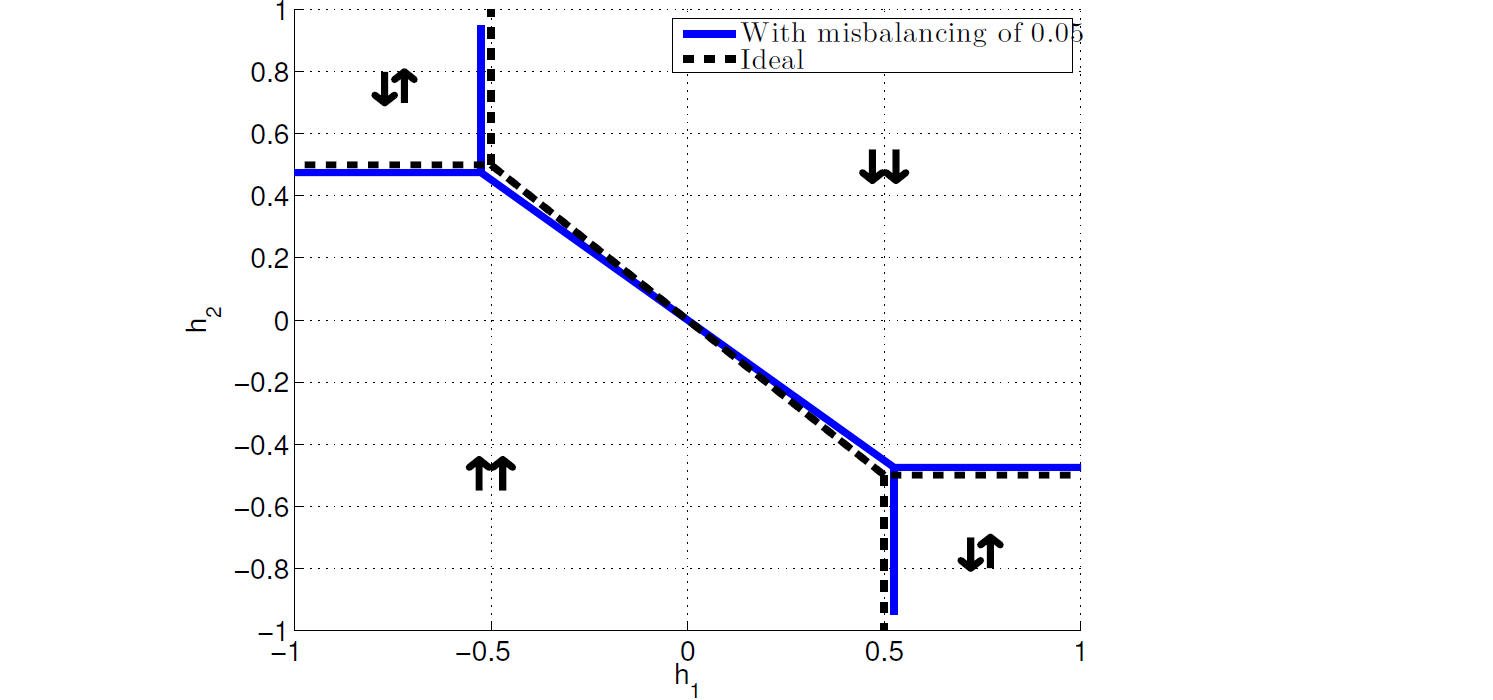
Fig. 101 Two-qubit (two Ising-spin) phase diagram for two spins of different magnitude (two qubits with different \(I_p\)) for a sample \(\chi\) value of \(J = -0.5\). The dashed lines show the locations of the expected phase boundaries between the four possible states of the system under the assumption of identical spin magnitudes. The solid lines show the locations of the phase boundaries for spin magnitudes that differ by \(0.05\). Data shown are representative of D-Wave 2X systems.

Characterizing the Effect of Flux Noise

This section characterizes the effects of flux noise on the quantum annealing process. The Error-Correction Features chapter describes the procedure that D-Wave uses to correct for drift.

Let there be a flux qubit biased at degeneracy \(h=0\) with tunneling energy \(\Delta_q\). Let the qubit be subject to flux noise with noise spectral density \(S_{\Phi}(f)\). If this qubit is subjected to experiments over a time interval \(t_{\rm exp}\), then it is subject to a random flux bias whose flux-flux correlator can be expressed as

\begin{equation} \left<\Phi_n(t)\Phi_n(0)\right> = \int_{f_{\rm min}}^{f_{\rm max}} df S_\Phi(f) \frac{\sin^2 2\pi f t}{(\pi f)^2} \end{equation}

where \(f_{\rm min} = 1/t_{\rm exp}\) and \(f_{\rm max} = \Delta_q/h\).[7]

[7]

The derivation of this expression follows the same logic as that for the phase-phase correlator given in Eq. 10c of Phys. Rev. B 67, 094510 (2003), albeit with an appropriate low-frequency cutoff.

The ambiguity with quantum annealing is in defining the appropriate choice of \(\Delta_q\), since this quantity is swept during an experiment. The value of \(\Delta_q\) should be the point in the anneal at which a given qubit localizes. For a single isolated qubit, the appropriate value of \(\Delta_q\) is on the order of the inverse decoherence time \(1/T_2^*\), where \(T_2^*\) is a function of \(\Delta_q\). Thus, \(\Delta_q\) becomes that of the coherent-incoherent crossover. For a system of coupled qubits, localization can occur at much larger values of \(\Delta_q\). In this case, the coupled qubit system can undergo a phase transition earlier in the anneal where the qubits are coherent. D-Wave QPUs realize these phase transitions at \(\Delta_q/h \sim 2\) GHz.

For example, the calculation of the fractional error in the dimensionless 1-local bias \(h_i\) proceeds as follows. Typical qubits experience low-frequency flux noise characterized by a noise spectral density of the form

\begin{equation} S_\Phi(f) = \frac{A}{f^\alpha} \end{equation}

with amplitude such that \({\sqrt S_\Phi ({\rm 1 Hz}) \sim 2 \mu\Phi_0/\sqrt{\rm Hz}}\) and exponent \(0.75 \leq \alpha < 1\). Given that the uncertainty in \(\alpha\) is large and a lack of experimental evidence that the form given above is valid up to frequencies of order \(\Delta_q/h \sim 2\) GHz, \(\alpha = 1\) is used in these calculations. Integrating this equation from \(f_{\rm min} = 1\) mHz to \(f_{\rm max} = 2\) GHz yields an integrated flux noise

\begin{equation} \delta \Phi_n = \sqrt{\int_{f_{\rm min}}^{f_{\rm max}} df S_\Phi(f)} \approx 10\ \mu\Phi_0. \end{equation}

A qubit with \(\Delta_q/h = 2\) GHz also possesses a persistent current \(|I_p| \approx 0.8\) \(\mu\)A. The maximum achievable antiferromagnetic coupling between a pair of qubits is \(M_{\rm AFM} \approx 2 \ {\rm pH}\). Thus, the scale of \(h\) is set by

\begin{equation} \Phi_h \equiv M_{\rm AFM} |I_p| \approx 0.8 \ {\rm m} \Phi_0. \end{equation}

The relative error in the dimensionless parameter \(h_i\) is then

\begin{equation} \delta h_i \equiv \frac{\delta \Phi_n}{\Phi_h} \approx 0.01. \end{equation}

Example of ICE Effects on Solution Quality

As discussed in the Sources of ICE section, the distributions \(\delta h\) and \(\delta J\) depend on annealing time \(t_f\) and vary with anneal fraction \(s\) during the anneal. Because \(\delta h\) and \(\delta J\) may vary with \(s\) (as well as with any errors in the ratio \(h/J\)), ICE can drive a system across a phase boundary—whether a quantum phase transition or a later classical phase transition.

Consider a simple two-spin problem with biases \(h_1 = h_2 = 0.01\) and \(J = -0.5\). You can expect to see spins \(\downarrow \downarrow\) (that is, \(s_1, s_2 = -1\)) in the problem solution. If \(\delta h\) is such that the QPU sees \(h_1, h_2 = -0.01\) early in the anneal, the system localizes in the \(\uparrow \uparrow\) state. Perhaps later, the effective ICE signal becomes smaller and the system crosses a phase boundary to prefer \(\downarrow \downarrow\). Depending on when this happens in relation to freezeout time, the system may or may not be able to respond:

• If \(\delta h\) changes early enough in the anneal, the system can respond and provide the correct answer.

• If \(\delta h\) occurs too late, the early ICE is effectively locked in and both spins remain up.

This example shows that there are two components to ICE: the final error on the classical Ising spin system defined by equation (1), and the rest of the error contributing to a variation in the anneal path on the way to the final classical Hamiltonian. Depending on problem details, either of these effects may dominate—exchanging roles earlier, later, or at multiple times in the anneal.