Solver Properties

The properties that characterize behaviors and supported features of SAPI solvers[1] can be queried through SAPI. This chapter defines these properties[2].

[1]

Ocean software also provides classical solvers such as steepest descent that you can run locally. See the Ocean documentation for information on parameters of such solvers.

[2]

Ocean software classes such as the DWaveSampler class may include various other properties that are derived and stored client-side, not read from SAPI in the properties dict; for example, the dwave.cloud.solver.BaseSolver might derive an avg_load property. See the Ocean documentation for those properties.

The examples below use the following setup:

>>> from dwave.system import DWaveSampler, LeapHybridSampler, LeapHybridCQMSampler, LeapHybridDQMSampler
...
>>> qpu_advantage = DWaveSampler(solver={'topology__type': 'pegasus'})
>>> hybrid_bqm_sampler = LeapHybridSampler()
>>> hybrid_cqm_sampler = LeapHybridCQMSampler()     
>>> hybrid_dqm_sampler = LeapHybridDQMSampler()

anneal_offset_ranges

Array of ranges of valid anneal offset values, in normalized offset units, for each qubit. The negative values represent the largest number of normalized offset units by which a qubit’s anneal path may be delayed. The positive values represent the largest number of normalized offset units by which a qubit’s anneal path may be advanced.

Example

For the solver configured in the example setup above,

>>> qpu_advantage.properties["anneal_offset_ranges"][50:55]       
[[-0.6437569799443247, 0.5093937328282595],
 [-0.6409899716199288, 0.5697835920492209],
 [-0.6468663649068287, 0.5211452841036136],
 [-0.6435316809914349, 0.5011584701861175],
 [-0.6500326191157569, 0.5392206819650301]]

anneal_offset_step

Quantization step size of anneal offset values in normalized units.

Example

For the solver configured in the example setup above,

>>> qpu_advantage.properties["anneal_offset_step"]      
-0.00017565852000668507

anneal_offset_step_phi0

Quantization step size in physical units (annealing flux-bias units): \(\Phi_0\).

Example

For the solver configured in the example setup above,

>>> qpu_advantage.properties["anneal_offset_step_phi0"]           
1.486239425109832e-05

annealing_time_range

Range of time, in microseconds with a resolution of 0.01 \(\mu s\), possible for one anneal (read). The lower limit in this range is the fastest quench possible for this solver using the standard-anneal protocol. See also the fast_anneal_time_range.

Default annealing time is specified by the default_annealing_time property.

Example

For the solver configured in the example setup above,

>>> qpu_advantage.properties["annealing_time_range"]        
[0.5, 2000.0]

category

Type of solver; for example,

• qpu: Quantum computers such as the Advantage.

• hybrid: Quantum-classical hybrid; typically one or more classical algorithms run on the problem while outsourcing to a quantum processing unit (QPU) parts of the problem where it benefits most.

Example

For the solver configured in the example setup above,

>>> hybrid_bqm_sampler.properties["category"]
'hybrid'

chip_id

Name of the solver.

Example

For the solver configured in the example setup above,

>>> qpu_advantage.properties["chip_id"]             
'Advantage_system1.1'

couplers

Couplers in the working graph. A coupler contains two elements [q1, q2], where both q1 and q2 appear in the list of working qubits, in the range [0, num_qubits - 1] and in ascending order (i.e., q1 < q2). These are the couplers that can be programmed with nonzero \(J\) values.

Example

For the solver configured in the example setup above,

>>> qpu_advantage.properties["couplers"][:5]           
[[30, 31], [31, 32], [32, 33], [33, 34], [34, 35]]

default_annealing_time

Default time, in microseconds with a resolution of 0.01 \(\mu s\), for one anneal (read). You can change the annealing time for a given problem by using the annealing_time or anneal_schedule parameters, but do not exceed the upper limit given by the annealing_time_range or fast_anneal_time_range property.

Example

For the solver configured in the example setup above,

>>> qpu_advantage.properties["default_annealing_time"]        
20.0

default_programming_thermalization

Default time, in microseconds with a resolution of 0.01 \(\mu s\), that the system waits after programming the QPU for it to return to base temperature. This value contributes to the total qpu_programming_time, which is returned by SAPI with the problem solutions.

You can change this value using the programming_thermalization parameter.

Example

For the solver configured in the example setup above,

>>> qpu_advantage.properties["default_programming_thermalization"]   
1000.0

default_readout_thermalization

Default time, in microseconds with a resolution of 0.01 \(\mu s\), that the system waits after each state is read from the QPU for it to cool back to base temperature. This value contributes to the qpu_delay_time_per_sample field, which is returned by SAPI with the problem solutions.

Example

For the solver configured in the example setup above,

>>> qpu_advantage.properties["default_readout_thermalization"]   
0.0

extended_j_range

Extended range of values possible for the coupling strengths (quadratic coefficients), \(J\), for this solver. Strong negative couplings may be necessary for some embeddings; however, such chains may require additional calibration through the flux_biases parameter to compensate for biases introduced by strong negative couplings. See also per_qubit_coupling_range and per_group_coupling_range.

The auto_scale parameter, which rescales \(h\) and \(J\) values in the problem to use as much of the range of \(h\) (h_range) and the range of \(J\) (extended_j_range) as possible, enables you to submit problems with values outside these ranges and have the system automatically scale them to fit.

Example

For the solver configured in the example setup above,

>>> qpu_advantage.properties["extended_j_range"]
[-2.0, 1.0]

fast_anneal_time_range

Range of time, in microseconds with a resolution of up to 1 ps[3], possible for one anneal (read). The lower limit in this range is the fastest quench possible for this solver.

Default annealing time is specified by the default_annealing_time property.

[3]

The fast-anneal protocol supports a time granularity of about 0.05% of the anneal time. For annealing times of about 2 ns, the granularity is about 1 ps; for anneals of about 20 \(\mu s\), it is reduced to around 10 ns. Therefore, the high resolution specified here is relevant to the minimum value of the provided range.

Example

For the solver configured in the example setup above,

>>> from dwave.system import DWaveSampler
>>> qpu_advantage2 = DWaveSampler(solver={"topology__type": "zephyr"}   
>>> qpu_advantage2.properties["fast_anneal_time_range"]        
[0.005, 2000.0]

h_gain_schedule_range

Range of the time-dependent gain applied to qubit biases for this solver.

Example

For the solver configured in the example setup above,

>>> qpu_advantage.properties["h_gain_schedule_range"]        
[-4.0, 4.0]

h_range

Range of values possible for the qubit biases (linear coefficients), \(h\), for this solver.

The auto_scale parameter, which rescales \(h\) and \(J\) values in the problem to use as much of the range of \(h\) (h_range) and the range of \(J\) (extended_j_range) as possible, enables you to submit problems with values outside these ranges and have the system automatically scale them to fit.

Example

For the solver configured in the example setup above,

>>> qpu_advantage.properties["h_range"]
[-4.0, 4.0]

j_range

Range of values possible for the coupling strengths (quadratic coefficients), \(J\), for this solver.

See also the extended_j_range solver property.

Example

For the solver configured in the example setup above,

>>> qpu_advantage.properties["j_range"]               
[-1.0, 1.0]

max_anneal_schedule_points

Maximum number of points permitted in a PWL waveform submitted to change the default anneal schedule.

For reverse annealing, the maximum number of points allowed is one more than the number given in the max_anneal_schedule_points property.

Example

For the solver configured in the example setup above,

>>> qpu_advantage.properties["max_anneal_schedule_points"]   
12

max_h_gain_schedule_points

Maximum number of points permitted in a PWL waveform submitted to set a time-dependent gain on linear coefficients (qubit biases, see the h parameter) in the Hamiltonian.

Example

For the solver configured in the example setup above,

>>> qpu_advantage.properties["max_h_gain_schedule_points"]     
20

maximum_number_of_biases

Maximum number of biases, both linear and quadratic in total, accepted by the solver.

Example

For the solver configured in the example setup above,

>>> hybrid_bqm_sampler.properties["maximum_number_of_biases"]    
200000000

maximum_number_of_cases

Maximum number of cases accepted by the solver.

For more details about cases and their role in DQMs, see the section on the DQM concept in the Ocean documentation.

Example

For the solver configured in the example setup above,

>>> hybrid_dqm_sampler.properties["maximum_number_of_cases"]    
500000

maximum_number_of_constraints

Maximum number of constraints accepted by the solver.

Example

For the solver configured in the example setup above,

>>> hybrid_cqm_sampler.properties["maximum_number_of_constraints"]   
100000

maximum_number_of_linear_biases_real

Maximum number of linear biases of type floating-point/real numbers counted across all constraints and the model’s objective.

Example

For the solver configured in the example setup above,

>>> hybrid_cqm_sampler.properties["maximum_number_of_linear_biases_real"]   
75000000

maximum_number_of_quadratic_variables

Maximum number of variables that have interactions (quadratic biases)—counted across all constraints (meaning that the same variable can be counted multiple times if it appears in interactions in more than one constraint)—accepted by the solver.

Example

For the solver configured in the example setup above,

>>> hybrid_cqm_sampler.properties["maximum_number_of_quadratic_variables"]   
15000000

maximum_number_of_quadratic_variables_real

Maximum number of variables that have interactions (quadratic biases) of type floating-point/real numbers—counted across all constraints (meaning that the same variable can be counted multiple times if it appears in interactions in more than one constraint)—accepted by the solver.

Example

For the solver configured in the example setup above,

>>> hybrid_cqm_sampler.properties["maximum_number_of_quadratic_variables_real"]   
0

maximum_number_of_variables

Maximum number of problem variables accepted by the solver.

Example

For the solver configured in the example setup above,

>>> hybrid_bqm_sampler.properties["maximum_number_of_variables"]    
1000000

maximum_time_limit_hrs

Maximum allowed run time, in hours, that can be specified for the solver.

Example

For the solver configured in the example setup above,

>>> hybrid_bqm_sampler.properties["maximum_time_limit_hrs"]     
24.0

minimum_time_limit

Minimum required run time, in seconds, the solver must be allowed to work on the given problem. Specifies the minimum time as a piecewise-linear curve defined by a set of floating-point pairs. The second element is the minimum required time; the first element in each pair is some measure of the problem, dependent on the solver:

• For hybrid BQM solvers, this is the number of variables.

• For hybrid DQM solvers, this is a combination of the numbers of interactions, variables, and cases that reflects the “density” of connectivity between the problem’s variables.

The minimum time for any particular problem is a linear interpolation calculated on two pairs that represent the relevant range for the given measure of the problem. For example, if minimum_time_limit for a hybrid BQM solver were [[1, 0.1], [100, 10.0], [1000, 20.0]], then the minimum time for a 50-variable problem would be 5 seconds, the linear interpolation of the first two pairs that represent problems with between 1 to 100 variables.

For more details, see the Ocean samplers documentation for solver methods that calculate this parameter, and their descriptions.

Example

For the solver configured in the example setup above,

>>> hybrid_bqm_sampler.properties["minimum_time_limit"]       
[[1, 3.0],
 [1024, 3.0],
 [4096, 10.0],
 [10000, 40.0],
 [30000, 200.0],
 [100000, 600.0],
 [1000000, 600.0]]

minimum_time_limit_s

Minimum required run time, in seconds, the solver must be allowed to work on any given problem.

For more details, see the Ocean samplers documentation for solver methods that calculate the default runtime of a given problem.

Example

For the solver configured in the example setup above,

>>> hybrid_cqm_sampler.properties["minimum_time_limit_s"]       
5

num_biases_multiplier

Multiplier used in the internal calculation of the minimum run time, minimum_time_limit_s, the solver must be allowed to work on the given problem.

Example

For the solver configured in the example setup above,

>>> hybrid_cqm_sampler.properties["num_biases_multiplier"]       
4.65705646e-06

num_constraints_multiplier

Multiplier used in the internal calculation of the minimum run time, minimum_time_limit_s, the solver must be allowed to work on the given problem.

Example

For the solver configured in the example setup above,

>>> hybrid_cqm_sampler.properties["num_constraints_multiplier"]       
6.44385747e-09

num_qubits

Total number of qubits, both working and nonworking,[4] in the QPU.

[4]

The qubits property provides the indices of qubits in the QPU’s working graph, which are the qubits you can use for problem solving.

Example

For the solver configured in the example setup above,

>>> qpu_advantage.properties["num_qubits"]               
5760

num_reads_range

Range of values possible for the number of reads that you can request for a problem.

Example

For the solver configured in the example setup above,

>>> qpu_advantage.properties["num_reads_range"]
[1, 10000]

num_variables_multiplier

Multiplier used in the internal calculation of the minimum run time, minimum_time_limit_s, the solver must be allowed to work on the given problem.

Example

For the solver configured in the example setup above,

>>> hybrid_cqm_sampler.properties["num_variables_multiplier"]       
0.000157411458

parameters

List of the parameters supported for the solver.

Example

For the solver configured in the example setup above,

>>> hybrid_bqm_sampler.properties["parameters"]             
{'time_limit': 'Maximum requested runtime in seconds.'}

per_group_coupling_range

Coupling range permitted per group of qubits for this solver. The couplers of every qubit are divided into two similar sized groups to which apply limitations on the total of all coupling strengths.

Strong negative couplings may be necessary for some embeddings, and can be enabled by using the extended_j_range range of \(J\) values. However, total \(J\) values of the couplers for a group of qubits must not exceed the range specified by this property. Also, chains may require additional calibration through the flux_biases parameter to compensate for biases introduced by strong negative couplings.

The auto_scale parameter scales a problem’s \(J\) values such that the total \(J\) values of the couplers for a group of qubits is within the range specified by this property.

For more information, see the Ocean documentation’s coupling_groups function.

Example

>>> from dwave.system import DWaveSampler
>>> qpu_advantage2 = DWaveSampler(solver={"topology__type": "zephyr"}   
>>> qpu_advantage2.properties["per_group_coupling_range"]        
[-13.000 10.000]

per_qubit_coupling_range

Coupling range permitted per qubit for this solver.

Strong negative couplings may be necessary for some embeddings, and can be enabled by using the extended_j_range range of \(J\) values. However, the total \(J\) values of the couplers for a qubit must not exceed the range specified by this property. Also, chains may require additional calibration through the flux_biases parameter to compensate for biases introduced by strong negative couplings.

The auto_scale parameter scales a problem’s \(J\) values such that the total \(J\) values of the couplers for a qubit is within the range specified by this property.

Example

For the solver configured in the example setup above,

>>> qpu_advantage.properties["per_qubit_coupling_range"]        
[-18.0, 15.0]

problem_run_duration_range

Range of time, in microseconds with a resolution of 0.01 \(\mu s\), that a submitted problem is allowed to run.

For details about how the run-duration limit is calculated, see QMI Runtime Limit.

Example

For the solver configured in the example setup above,

>>> qpu_advantage.properties["problem_run_duration_range"]       
[0.0, 1000000.0]

problem_timing_data

Key-value pairs that contain sample timing data and specify the version 1.0.x problem-timing model used to estimate problem runtimes for a QPU solver. For details about using the timing data to estimate the QPU access times for problem submissions, see the Estimating Access Time section.

The key-value pairs are the following:

• decorrelation_max_nominal_anneal_time: Parameter, in microseconds, used in the calculation of inter-sample correlation time. For more information, see the reduce_intersample_correlation solver property.

• decorrelation_time_range: Range of inter-sample correlation time, in microseconds, to add to the per-sample delay time as specified in the qpu_delay_time_per_sample field. Scales linearly with the anneal time from 0 to the amount returned in the decorrelation_max_nominal_anneal_time field. For more details, see the reduce_intersample_correlation solver parameter.

• default_annealing_time: See the default_annealing_time solver property.

• default_programming_thermalization: See the default_programming_thermalization solver property.

• default_readout_thermalization: See the default_readout_thermalization solver property.

• qpu_delay_time_per_sample: Default for the per-sample delay time in microseconds.

• readout_time_model: The readout-time model used to generate the set of data points; these data points define a piecewise-linear curve of typical readout times as a function of the number of qubits in a representative set of problems embedded on a QPU. The data points are provided in the readout_time_model_parameters field. Supported values that specify the scale of the curve are:

  • pwl_log_log: The log scale is used for both the horizontal and vertical axes.

  • pwl_linear: The linear scale is used for both the horizontal and vertical axes.

• readout_time_model_parameters: A set of \(2N\) data points generated by the readout-time model specified in the readout_time_model field.

• reverse_annealing_with_reinit_delay_time_delta: Extra per-sample delay time, in microseconds, when reverse annealing is used and the reinitialize_state parameter is true.

• reverse_annealing_with_reinit_prog_time_delta: Extra programming time, in microseconds, when reverse annealing is used and the reinitialize_state solver parameter is true.

• reverse_annealing_without_reinit_delay_time_delta: Extra per-sample delay time, in microseconds, when reverse annealing is used and the reinitialize_state solver parameter is false.

• reverse_annealing_without_reinit_prog_time_delta: Extra programming time, in microseconds, when reverse annealing is used and the reinitialize_state solver parameter is false.

• typical_programming_time: Typical programming time in microseconds.

• version: Version of the problem-timing model.

Example

For the solver configured in the example setup above,

>>> qpu_advantage.properties["problem_timing_data"]   
{'version': '1.0.0', 'typical_programming_time': 14072.88,
'reverse_annealing_with_reinit_prog_time_delta': 0.0,
'reverse_annealing_without_reinit_prog_time_delta': 5.55,
'default_programming_thermalization': 1000.0, 'default_annealing_time': 20.0,
'readout_time_model': 'pwl_log_log',
'readout_time_model_parameters': [0.0, 0.7699665876947938, 1.7242758696010096,
2.711975459489206, 3.1639057672764026, 3.750276915153992, 1.539131714800995,
1.8726623164229292, 2.125631787097315, 2.332672340068556, 2.371606651233025,
2.3716219271760215], 'qpu_delay_time_per_sample': 20.54,
'reverse_annealing_with_reinit_delay_time_delta': -4.5,
'reverse_annealing_without_reinit_delay_time_delta': -1.5,
'default_readout_thermalization': 0.0, 'decorrelation_max_nominal_anneal_time': 2000.0,
'decorrelation_time_range': [500.0, 10000.0]}

programming_thermalization_range

Range of time, in microseconds with a resolution of 0.01 \(\mu s\), possible for the system to wait after programming the QPU for it to cool back to base temperature. This value contributes to the total qpu_programming_time, which is returned by SAPI with the problem solutions.

You can change this value using the programming_thermalization parameter, but be aware that values lower than the default accelerate solving at the expense of solution quality.

Default value for a solver is given in the default_programming_thermalization property.

Example

For the solver configured in the example setup above,

>>> qpu_advantage.properties["programming_thermalization_range"]   
[0.0, 10000.0]

qubits

Indices of the working graph.

In a D-Wave QPU, the set of qubits and couplers that are available for computation is known as the working graph. The working graph typically does not contain all the qubits and couplers that are fabricated and physically present in the QPU. For example, an Advantage with its 5760 qubits (the num_qubits property), of which a maximum of 5640 are calibrated for problem solving (the programmable fabric, or largest component of the full Pegasus graph), might have a working graph of 5627 qubits (a yield of 99.7%) due to 13 qubits that were not brought into a consistent parametric regime in the calibration process. For such a system, the value of the qubits property is the sequence of integers between 30, the first of the 5640 fabric qubits, and 5729, the last of those 5640 qubits, minus indices of the 13 non-working qubits.[5]

[5]

You can see the qubit indexing scheme of such an Advantage QPU with Ocean’s dwave_networkx.pegasus_graph() function, which enables you to generate Pegasus graphs.

Example

For the solver configured in the example setup above,

>>> qpu_advantage.properties["qubits"][:5]         
[30, 31, 32, 33, 34]

quota_conversion_rate

Rate at which user or project quota is consumed for the solver as a ratio to QPU solver usage. Different solver types may consume quota at different rates.

Time is deducted from your quota according to:

\[\frac{num\_seconds}{quota\_conversion\_rate}\]

See the QPU Solver Datasheet guide for more information.

Example

For the solver configured in the example setup above,

>>> hybrid_bqm_sampler.properties["quota_conversion_rate"]
1

readout_thermalization_range

Range of time, in microseconds with a resolution of 0.01 \(\mu s\), possible for the system to wait after each state is read from the QPU for it to cool back to base temperature. This value contributes to the qpu_delay_time_per_sample field, which is returned by SAPI with the problem solutions.

Default readout thermalization time is specified in the default_readout_thermalization property.

Example

For the solver configured in the example setup above,

>>> qpu_advantage.properties["readout_thermalization_range"]       
[0.0, 10000.0]

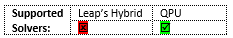
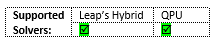
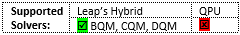
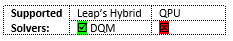
supported_problem_types

Indicates what problem types are supported for the solver.

QPU solvers support the following energy-minimization problem types:

• qubo: Quadratic unconstrained binary optimization (QUBO) problems; use \(0/1\)-valued variables.

• ising: Ising model problems; use \(-1/1\)-valued variables.

Hybrid solvers support the following energy-minimization problem types:

• bqm: Binary quadratic model (BQM) problems; use \(0/1\)-valued variables and \(-1/1\)-valued variables; constraints are typically represented as penalty models.

• cqm: Constrained quadratic model (CQM) problems; use both binary-valued variables (both \(0/1\)-valued variables and \(-1/1\)-valued variables) and integer-valued variables; support constraints natively.

• dqm: Discrete quadratic model (DQM) problems; use variables that can represent a set of values such as {red, green, blue, yellow} or {3.2, 67}; constraints are typically represented as penalty models.

Example

For the solver configured in the example setup above,

>>> qpu_advantage.properties["supported_problem_types"]       
['ising', 'qubo']

tags

May hold attributes about a solver that you can use to have a client program choose one solver over another.

Example

For the solver configured in the example setup above,

>>> qpu_advantage.properties["tags"]          
[]

topology

Indicates the topology type (pegasus or zephyr) and shape of the QPU graph.

Example

The topology seen in this example is a P16 Pegasus graph. See the D-Wave QPU Architecture: Topologies section of the Getting Started with D-Wave Solvers guide for a description of QPU topologies.

For the solver configured in the example setup above,

>>> qpu_advantage.properties["topology"]                    
{'type': 'pegasus', 'shape': [16]}

version

Version number of the solver.

Example

For the solver configured in the example setup above,

>>> hybrid_bqm_sampler.properties["version"]                 
'2.0'

vfyc

Obsolete property that is always False.

Example

For the solver configured in the example setup above,

>>> qpu_advantage.properties["vfyc"]              
False