Appendix: Next Learning Steps

The previous chapters presented a high-level explanation of solving problems on D-Wave solvers, using an intuitive approach. This chapter starts you off on your journey to mastering more methodical techniques.

Problem Formulation

To map a problem to a quadratic model, you can try the following steps.

1. Write out the objective and constraints.

   This should be written out in terms of your problem domain, not necessarily in math format.

   • The objective of a problem is what you are looking to minimize[1].

   • A constraint in a problem is a rule that you must follow; an answer that does not satisfy a given constraint is called infeasible, it’s not a good answer, and might not be usable at all. For example, a travelling salesperson cannot be in two cities at once or the trucks in your problem may not be able to hold more than 100 widgets.

   There may be more than one way to interpret your problem in terms of objectives and constraints.

2. Convert objective and constraints into math expressions.

   Decide on the type of variables to best formulate it:

   • Binary

     Does your application optimize over decisions that could either be true (or yes) or false (no)? For example,

     • Should the antenna transmit or no?

     • Did a network node experience failure?

   • Discrete

     Does your application optimize over several distinct options? For example,

     • Which shift should employee X work?

     • Should the state be colored red, blue, green or yellow?

   • Integer

     Does your application optimize the number of something? For example,

     • How many widgets should be loaded onto the truck?

   • Continuous

     Does your application optimize over an uncountable set? For example,

     • Where should the sensor be built?

   Once you think of a problem in these terms, you can assign a variable for each question.

   Next ask about the degree the problem can likely be formulated as:

   • Quadratic

     Are its relationships defined pairwise? For example,

     • In the structural imbalance example each pair of people in the network is either friendly or hostile.

   • Higher-Order

     Does your application have relationships between multiple variables at once? For example,

     • Simulating an AND gate

   Next, transform objective and constraints into math expressions. For binary variables, this can often be done with truth tables if you can break the problem down into two- or three-variable relationships. For other variables and non-quadratic degrees, you can try techniques such as Non-Quadratic (Higher-Degree) Polynomials and Ocean tools such as Higher-Order Models.

3. Reformulate as a quadratic model.

   Different types of expressions require different strategies. Expressions derived from truth tables may not need any adjustments. The D-Wave Problem-Solving Handbook provides a variety of reformulation techniques; some common reformulations are:

   • Squared terms: QUBO and Ising models do not have squared binary variables. In QUBO format, its 0 and 1 values remain unchanged when squared, so you can replace any term \(x_i^2\) with \(x_i\). In Ising format, its -1 and +1 values always equal 1 when squared, so you can replace any term \(s_i^2\) with the constant 1.

   • Maximization to minimization: if your objective function is a maximization function (for example, maximizing profit), you can convert this to a minimization by multiplying the entire expression by -1. For example:

     \[\mbox{arg max} (3v_1+2v_1v_2) = \mbox{arg min} (-3v_1-2v_1v_2)\]

   • Equality to minimization: if you have a constraint that is an equality, you can convert it to a minimization expression by moving all arguments and constants to one side of the equality and squaring the non-zero side of the equation. This leaves an expression that is satisfied at its smallest value (0) and unsatisfied at any larger value (>0). For example, the equation \(x+1=2\) can be converted to \(\min_x[2-(x+1)]^2\), which has a minimum value of zero for the solution of the equation, \(x=1\).

     This approach is useful also for \(n \choose k\) constraints (selection of exactly \(k\) of \(n\) variables), where you disfavor selections of greater or fewer than \(k\) variables with the penalty \(P = \alpha (\sum_{i=1}^n x_i - k)^2\), where \(\alpha\) is a weighting coefficient (see penalty method) used to set the penalty’s strength.

4. Combine expressions.[2]

   Once you have written all of the components (objective and constraints) as quadratic models, for example BQMs, make a final BQM by adding all of the components. Typically you multiply each expression by a constant that weights the different constraints against each other to best reflect the requirements of your problem. You may need to tune these multipliers through experimentation to achieve good results. You can see examples in Ocean software’s collection of code examples on GitHub.

[1]

For maximization see step 3.

[2]

When using penalty models for constraints.

Example: Formulate an Ising Model

This example returns to the simple SAT of the Unconstrained Example: Solving a SAT Problem chapter but posed as a constraint and formulated as an Ising model following the steps above.

The problem now is to formulate a BQM that represents “the value of \(v_1\) should be identical to the value of \(v_2\)”, where \(v_1\) and \(v_2\) are binary-valued variables.[3]

[3]

This could be one small part of a larger problem, for example, an integer_factorization problem formulated with Boolean gates, as demonstrated in the Leap demo and Factoring Jupyter Notebook. The larger problem is to satisfy a constraint that two variables representing factors be assigned values such that their multiplication equals the factored number. The constraint of this section’s example might represent a connection between two gates of such a formulation of the factoring problem.

Step 1 is to state just a constraint, \(v_1\) equals \(v_2\).

Step 2 is just to write the constraint as either an equation or a truth table (the problem’s variables are already binary valued).

This example shows both: the constraint as an equation is simply, \(v_1 = v_2\), and below it is represented as a truth table (notice that for an Ising formulation the values are \(\{-1, 1\}\) rather than \(\{0, 1\}\)).

State	\(v_1\)	\(v_2\)	\(v_1 = v_2\)
1	-1	-1	True
2	-1	1	False
3	1	-1	False
4	1	1	True

Step 3 here also demonstrates reformulating for both expressions. First, note that for two variables, the Ising Model formulation reduces to,

\[\text{E}(h_i, J_{i,j}; S_i) = h_1 s_1 + h_2 s_2 + J_{1,2} s_1 s_2.\]

Reformulating the equality expression as a minimization can be done as follows:

\[v_1 = v_2 \qquad \rightarrow \qquad \min_v[v_1 - v_2]^2\]

Expanding the square gives,

\[\begin{split}\min_v[v_1 - v_2]^2 &= \min_v[v_1^2 + v_2^2 - 2v_1v_2] \\ &= \min_v[1 + 1 -2v_1v_2] \\ &= \min_v[2 -2v_1v_2]\end{split}\]

You can now map the minimization directly to \(-2 s_1 s_2\), dropping the constant.

Notice that for this Ising model the energy gap between the ground states (e.g., \(E(s_1=s_2=-1)=-2\)) and the excited states (e.g., \(E(s_1=-1, s_2=+1)=+2\)) is 4. If you want a gap of 1, your Ising model is \(E(s_1, s_2) = -0.5 s_1 s_2\).

Alternatively, if you prefer a truth table, you can reformulate as a penalty function. Here, an energy gap of 1 is chosen.

State	\(v_1\)	\(v_2\)	Penalty
1	-1	-1	p
2	-1	1	p+1
3	1	-1	p+1
4	1	1	p

Substituting the values of the table’s variables for variables \(s_1, s_2\) in the two-variable Ising model above, and the desired penalty for the resulting energy, produces for the four rows of the table these four equalities:

\[\begin{split}\text{State 1} \qquad h_1 (-1) + h_2 (-1) + J_{1,2} (-1) (-1) &= p \\ \text{State 2} \qquad h_1 (-1) + h_2 (+1) + J_{1,2} (-1) (+1) &= p+1 \\ \text{State 3} \qquad h_1 (+1) + h_2 (-1) + J_{1,2} (+1) (-1) &= p+1 \\ \text{State 4} \qquad h_1 (+1) + h_2 (+1) + J_{1,2} (+1) (+1) &= p\end{split}\]

Giving the following four equations with four variables:

\[\begin{split}-h_1 - h_2 + J_{1,2} &= p \\ -h_1 + h_2 - J_{1,2} &= p+1 \\ h_1 - h_2 - J_{1,2} &= p+1 \\ h_1 + h_2 + J_{1,2} &= p\end{split}\]

Solving these equations[4] gives \(E(s_1, s_2) = -0.5 s_1 s_2\).

[4]

Adding the first and fourth equation immediately gives \(J_{1,2} = p\). Adding the second and third, and replacing \(J_{1,2}\) for \(p\), gives \(J_{1,2} = p = -0.5\). Adding the first two equations, with these now-known values, produces \(h_1 = h_2 = 0\).

Submitting for solution on a D-Wave quantum computer is similar to the submission shown in the Constraints Example: Submitting to a QPU Solver chapter, where it was done for QUBOs:

>>> from dwave.system import DWaveSampler, EmbeddingComposite
>>> sampler = EmbeddingComposite(DWaveSampler())
...
>>> h = {}
>>> J = {('s1', 's2'): -0.5}
>>> sampleset = sampler.sample_ising(h, J, num_reads=1000)
>>> print(sampleset)                    
  s1 s2 energy num_oc. chain_.
0 -1 -1   -0.5     372     0.0
1 +1 +1   -0.5     628     0.0
['SPIN', 2 rows, 1000 samples, 2 variables]

Next Steps for Learning to Formulate Problems

You can learn more about formulating problems here:

• Problem Formulation Guide on the D-Wave corporate website

• D-Wave Problem-Solving Handbook

• Ocean software’s collection of code examples on GitHub.

• D-Wave’s Quantum Programming - Core Training

Ising and QUBO Formulations

Figure 37 compares Ising and QUBO notation and related terminology.

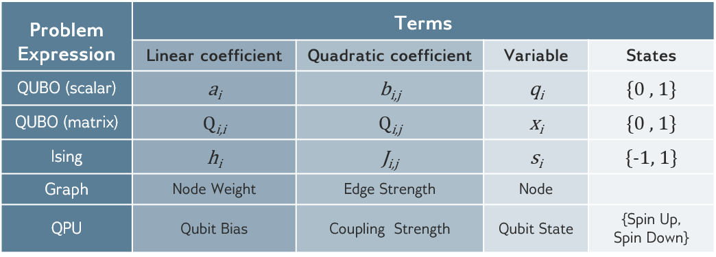
Fig. 37 Notation conventions.

Some problems may be easier to formulate or see better results with Ising over QUBO, and vice versa. As demonstrated in the interactive code examples of the Leap demo and Structural Imbalance Jupyter Notebook, the structural balance of signed social networks[5] is easily modeled in Ising format:

\[\sum_{i<j}^N J_{i,j} s_i s_j\]

[5]

Social networks map relationships between people or organizations onto graphs, with the people/organizations as nodes and relationships as edges; for example, Facebook friends form a social network. Signed social networks map both friendly and hostile relationships by assigning to edges either positive or negative values. Such networks are said to be structurally balanced when they can be cleanly divided into two sets, with each set containing only friends, and all relations between these sets are hostile.

Transformations Between Ising and QUBO

The transformation between these formats is trivial:

\[s = 2x - 1.\]

Example of Transforming a QUBO to Ising Format

Use \(x_i \mapsto \frac{s_i +1}{2}\) to translate a QUBO model to an Ising model, as here:

\[\begin{split}\begin{array}{rcl} f(x) &=& -22x_1 - 6x_2 - 14x_3 + 20x_1x_2 + 28x_1x_3 + 9 \\ \tilde{f}(s) &=& -22 \left( \frac{s_1+1}{2} \right) - 6 \left( \frac{s_2+1}{2} \right) - 14 \left(\frac{s_3+1}{2} \right) \\ & & + 20 \left(\frac{s_1+1}{2} \right) \left( \frac{s_2+1}{2} \right) + 28 \left( \frac{s_1+1}{2} \right) \left( \frac{s_3+1}{2} \right) + 9 \\ &=& -11s_1-11 - 3s_2-3 - 7s_3-7 + 5s_1s_2 + 5s_1 + 5s_2 +5 + 7s_1s_3 \\ & & + 7s_1 + 7s_3 + 7 + 9 \\ &=& s_1 + 2s_2 + 5s_1s_2 + 7s_1s_3 \end{array}\end{split}\]

Ocean software can automate such conversion for you:

>>> import dimod
>>> dimod.qubo_to_ising({('x1', 'x1'): -22, ('x2', 'x2'): -6, ('x3', 'x3'): -14,
...                      ('x1', 'x2'): 20, ('x1', 'x3'): 28},
...                      offset=9)
({'x1': 1.0, 'x2': 2.0, 'x3': 0.0}, {('x1', 'x2'): 5.0, ('x1', 'x3'): 7.0}, 0.0)

Example of Transforming a Ising to QUBO Format

Use \(s_i \mapsto 2x_i -1\) to translate an Ising model to a QUBO model, as here:

\[\begin{split}\begin{array}{rcl} g(s) &=& s_1 + 2s_2 + 5s_1s_2 + 7s_1s_3 \\ \tilde{g}(x) &=& (2x_1 - 1) + 2(2x_2 - 1) + 5(2x_1 - 1)(2x_2 - 1) \\ & & + 7(2x_1 - 1)(2x_3 - 1)\\ &=& 2x_1 - 1 + 4x_2 - 2 + 20x_1x_2 - 10x_1 - 10x_2 + 5 + 28x_1x_3 - 14x_1 \\ & & - 14x_3 + 7 \\ &=& - 22x_1 - 6x_2 - 14x_3 + 20x_1x_2 + 28x_1x_3 + 9 \end{array}\end{split}\]

Using Ocean software:

>>> import dimod
>>> dimod.ising_to_qubo({'s1': 1, 's2': 2}, {('s1', 's2'): 5, ('s1', 's3'): 7}) 
({('s1', 's1'): -22.0, ('s2', 's2'): -6.0, ('s1', 's2'): 20.0,
  ('s1', 's3'): 28.0, ('s3', 's3'): -14.0},
  9.0)

Next Steps for Learning about Problem Formats

You can learn more about the QPU’s native formulations in the D-Wave Problem-Solving Handbook.

Solver Parameters

In previous sections and chapters, you saw the use of parameters such as num_reads in submissions of problems to D-Wave solvers. Setting appropriate parameters can be both hard and crucial to finding good solutions.

num_reads

Consider the outcome of submitting the exactly-one-true constraint of the Constraints Example: Problem Formulation chapter without specifying the number of anneals.

from dwave.system import DWaveSampler, EmbeddingComposite
sampler = EmbeddingComposite(DWaveSampler())
Q = {('a', 'a'): -1, ('b', 'b'): -1, ('c', 'c'): -1,
     ('a', 'b'): 2, ('b', 'c'): 2, ('a', 'c'): 2}
sampleset = sampler.sample_qubo(Q)

The single run above returned a solution that is correct but incomplete in that it is one of three possible ground states:

>>> print(sampleset)                         
   a  b  c energy num_oc. chain_.
0  0  1  0   -1.0       1     0.0
['BINARY', 1 rows, 1 samples, 3 variables]

For harder problems, the number of anneals you request might determine whether or not you see correct or good solutions at all.

auto_scale

In the Unconstrained Example: Solving a SAT Problem chapter, you developed a QUBO for a simple SAT problem,

\[E(q_i) = 0.1 q_1 + 0.1 q_2 - 0.2 q_1 q_2,\]

where \(a_1 = a_2 = 0.1\) was set to an arbitrary positive number.

Consider now assigning a value of 0.5 to the qubit biases and likewise multiplying the coupler strength fivefold to -1, uniformly scaling the objective function by 5. The scaled QUBO is now,

\[E(q_i) = 0.5 q_1 + 0.5 q_2 - q_1 q_2\]

This objective function also favors states 0 and 4, but the objective value for the excited states is now 0.5 rather than 0.1 previously:

State	\(q_1\)	\(q_2\)	Objective Value
1	0	0	0
2	0	1	0.5
3	1	0	0.5
4	1	1	0

Recall that the previous objective function returned results that included a small fraction of excited states. One might expect that increasing the value (penalty) of the objective function for the excited states—enlarging the energy gap between the ground state and excited states—would make the excited states harder to reach and therefore less probable.

In fact problems submitted to a QPU solver can benefit from an autoscaling feature: each QPU has an allowed range of values for its qubit biases and coupler strengths (\(a\) and \(b\) in the QUBO format); by default, the system adjusts the \(a\) and \(b\) values of submitted problems to make use of the entire available range before configuring the QPU’s biases and coupler strengths.

You can explicitly disable autoscaling (auto_scale=False). Below are results for submitting both QUBOs with and without autoscaling.

>>> from dwave.system import DWaveSampler, EmbeddingComposite
>>> sampler = EmbeddingComposite(DWaveSampler())
...
>>> # Define QUBOs
>>> Q1 = {('q1', 'q1'): 0.1, ('q2', 'q2'): 0.1, ('q1', 'q2'): -0.2}
>>> Q2 = {('q1', 'q1'): 0.5, ('q2', 'q2'): 0.5, ('q1', 'q2'): -1}
...
>>> # Autoscaling on for original QUBO
>>> sampleset = sampler.sample_qubo(Q1, num_reads=5000)
>>> print(sampleset)                         
  q1 q2 energy num_oc. chain_.
0  0  0    0.0    2764     0.0
1  1  1    0.0    2233     0.0
2  0  1    0.1       1     0.0
3  1  0    0.1       2     0.0
['BINARY', 4 rows, 5000 samples, 2 variables]
...
>>> # Autoscaling on for scaled-up QUBO
>>> sampleset = sampler.sample_qubo(Q2, num_reads=5000)
>>> print(sampleset)                       
  q1 q2 energy num_oc. chain_.
0  0  0    0.0    3429     0.0
1  1  1    0.0    1570     0.0
2  0  1    0.5       1     0.0
['BINARY', 3 rows, 5000 samples, 2 variables]
...
>>> # Autoscaling off for original QUBO
>>> sampleset = sampler.sample_qubo(Q1, num_reads=5000, auto_scale=False)
>>> print(sampleset)                      
  q1 q2 energy num_oc. chain_.
0  0  0    0.0    1603     0.0
1  1  1    0.0    1669     0.0
2  0  1    0.1     824     0.0
3  1  0    0.1     904     0.0
['BINARY', 4 rows, 5000 samples, 2 variables]
...
>>> # Autoscaling off for scaled-up QUBO
>>> sampleset = sampler.sample_qubo(Q2, num_reads=5000, auto_scale=False)
>>> print(sampleset)                         
  q1 q2 energy num_oc. chain_.
0  0  0    0.0    2773     0.0
1  1  1    0.0    2000     0.0
2  1  0    0.5     103     0.0
3  0  1    0.5     124     0.0
['BINARY', 4 rows, 5000 samples, 2 variables]

With autoscaling (the default), the two problems are run on the QPU with the same qubit biases and coupling strengths and therefore return similar solutions. (The energies and objective values reported are for the pre-scaling values.) With autoscaling disabled, the first problem, with its smaller energy gap, returns more samples of the excited states.

chain_strength

Although not a parameter of D-Wave solvers, chain_strength—a parameter used by some Ocean tools submitting problems to quantum samplers—may also be crucial to successfully solving some problems.

The Constraints Example: Minor-Embedding chapter explained that for a chain of qubits to represent a variable, all its constituent qubits must return the same value for a sample, and that this is accomplished by setting a strong coupling to the edges connecting these qubits. It set a value that was a bit stronger than the coupler strength representing edges of the problem.

The last statement might have raised the question, Why not simply maximize the coupling strength for all qubits in all chains? Now, having learnt about the auto_scale parameter, you can understand the answer.

In the problem of the exactly-one-true constraint of the Constraints Example: Problem Formulation chapter, the values set for the problem were:

• qubit biases: -1 and 1,

• coupler strengths between qubits representing variables: 2

• coupler strength between qubits of a chain: -3

Consider a simplified QPU that has a range of -1 to 1 for both biases and coupler strengths. For the maximum value of -3 to fit into the range, it must be scaled down to -1 (i.e., divided by 3). The scaled problem programmed on such a QPU has values:

• qubit biases: \(\frac{-1}{3}\) and \(\frac{1}{3}\)

• coupler strengths between qubits representing variables: \(\frac{2}{3}\)

• coupler strength between qubits of a chain:-1

If you instead were to use a chain strength of -10, the programmed values are now:

• qubit biases: \(\frac{-1}{10}\) and \(\frac{1}{10}\)

• coupler strengths between qubits representing variables: \(\frac{2}{10}\)

• coupler strength between qubits of a chain:-1

Notice that the difference between positive and negative qubit biases has shrunk from \(\frac{2}{3}\) (\(\frac{1}{3}\) - \(\frac{-1}{3}\)) to just 0.2, and likewise the coupling between qubits representing variables. The QPU is not a high-precision digital computer, it is analog and noisy. For problems with a variety of values for its linear and quadratic coefficients, overly large chain strength degrades the problem definition.

Ocean software tries to set smart default values for your chain strengths. However, complex problems might require “tuning” of chain strengths to reach acceptable solution quality.

Ocean provides tools and information to help you find good values for chain strengths when its default values are inadequate.

For example, you might see information on broken chains (chains with qubits that are not all in a single state at the end of the anneal) in returned solutions; if a high percentage of results have broken chains, you might need to increase the coupler strengths; if no or few chains are broken, possibly chain strengths are too strong.

Ocean’s problem inspector is a tool for visualizing problems submitted to, and answers received from, D-Wave systems. It helps you see the chains and potential problems.

num_spin_reversal_transforms

Although not a parameter of D-Wave solvers, num_spin_reversal_transforms—a parameter used by Ocean software’s SpinReversalTransformComposite composite when submitting problems to quantum samplers—may be very helpful to performance on some problems.

Notice that the results shown in the auto_scale section above tend to display some asymmetry between the two valid solutions. Qubits on a QPU can be biased to some small degree in one direction or another. The Spin-Reversal (Gauge) Transforms section of the D-Wave Problem-Solving Handbook guide, explains how spin-reversal transforms can improve results by reducing the impact of analog errors that may exist on the QPU.

>>> from dwave.system import DWaveSampler, EmbeddingComposite
>>> from dwave.preprocessing import SpinReversalTransformComposite
...
>>> sampler = EmbeddingComposite(SpinReversalTransformComposite(DWaveSampler()))
...
>>> Q1 = {('q1', 'q1'): 0.1, ('q2', 'q2'): 0.1, ('q1', 'q2'): -0.2}
>>> sampleset = sampler.sample_qubo(Q1, num_reads=500, num_spin_reversal_transforms=10)
>>> print(sampleset.aggregate())                                  
q1 q2 energy num_oc. chain_.
0  0  0    0.0    2538     0.0
1  1  1    0.0    2461     0.0
2  1  0    0.1       1     0.0
['BINARY', 3 rows, 5000 samples, 2 variables]

The rerunning of one of the auto_scale section’s submissions above produced results that are more symmetrical in this case. The use of this composite has a cost of longer runtime.

Next Steps for Learning about Solver Parameters

Once you have submitted a few first problems of your own to D-Wave solvers, and you are ready to ensure your submissions are configured to produce the best solutions, familiarize yourself with the solver parameters.

You can learn more about solver parameters here:

• Solver Properties and Parameters Reference

• QPU Solver Datasheet to understand the cost increasing num_reads might have for real-time applications.

• D-Wave Problem-Solving Handbook and QPU Solver Datasheet guides provide more advanced information on D-Wave systems and best practices.

Next Learning Steps

Your next learning steps in general depends on how you prefer to learn. Below are some options:

Software

If your preferred learning approach is through programming, consider starting with these resources:

• Ocean software’s Getting Started documentation provides a series of code examples, for different levels of experience, that explain various aspects of quantum computing in solving problems.

• Ocean software’s collection of code examples on GitHub.

Hardware

If you want to better understand the D-Wave quantum computer system, start with these system-documentation guides:

• Technical details about the system: QPU Solver Datasheet.

• The D-Wave Problem-Solving Handbook guide’s bibliography is a good starting place for papers on quantum computing.

• Solver Properties and Parameters Reference

Training

If you prefer hands-on practice with instructor support, consider registering for D-Wave’s Quantum Programming - Core training.

Additional Resources

See also D-Wave corporate website for papers and links to user applications.