Problem Parameters#
The problems you send to D‑Wave solvers
include problem parameters (e.g., linear biases, h, of an
Ising problem) and solver parameters that control how
the problem is run (e.g., an annealing schedule, anneal_schedule).
Ocean software tools and SAPI’s
REST API provide various abstractions for
encoding the linear and quadratic biases that configure problems on D‑Wave
QPUs and enable expansion to problems such as the
constrained quadratic model (CQM)
and the nonlinear model solved on the
hybrid solvers in the Leap service.
For example, Ocean software’s DWaveSampler accepts
problems as a BinaryQuadraticModel, which contains both the
Q of the QUBO format and h and J of the
Ising format, as well as the latter three directly; e.g.,
DWaveSampler().sample_qubo(Q) and DWaveSampler().sample_ising(h, J)
and DWaveSampler().sample(bqm).
This chapter describes the problem parameters accepted by D‑Wave solvers, in alphabetical order.
bqm#
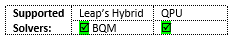
Ocean software’s dimod.binary.BinaryQuadraticModel (BQM) contains
linear and quadratic biases for problems formulated as
binary quadratic models as well as
additional information such as variable labels and offset.
For QPU solvers, Ocean software converts to Ising format and submits linear and quadratic biases.
Relevant Properties#
maximum_number_of_variables defines the maximum number of problem variables for hybrid solvers.
maximum_number_of_biases defines the maximum number of problem biases for hybrid solvers.
minimum_time_limit and maximum_time_limit_hrs define the runtime duration for hybrid solvers.
Example#
This example creates a BQM from a QUBO and submits it to a QPU.
>>> import dimod
>>> from dwave.system import DWaveSampler, EmbeddingComposite
...
>>> Q = {(0, 0): -3, (1, 1): -1, (0, 1): 2, (2, 2): -1, (0, 2): 2}
>>> bqm = dimod.BQM.from_qubo(Q)
>>> sampleset = EmbeddingComposite(DWaveSampler()).sample(bqm, num_reads=100)
cqm#
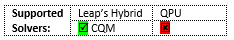
Ocean software’s dimod.ConstrainedQuadraticModel (CQM) contains linear
and quadratic biases for problems formulated as
constrained quadratic models as well as
additional information such as variable labels, offsets, and equality and
inequality constraints.
Relevant Properties#
maximum_number_of_variables defines the maximum number of problem variables for hybrid solvers.
maximum_number_of_biases and maximum_number_of_quadratic_variables define the maximum number of problem biases for hybrid solvers.
maximum_number_of_constraints defines the maximum number of constraints accepted by the solver.
minimum_time_limit_s and maximum_time_limit_hrs define the runtime duration for hybrid solvers.
num_biases_multiplier, num_constraints_multiplier, and num_variables_multiplier define multipliers used in the internal calculation of the default run time for a given problem.
Example#
This example creates a single-constraint CQM and submits it to a CQM solver.
>>> from dimod import ConstrainedQuadraticModel, Binary
>>> from dwave.system import LeapHybridCQMSampler
...
>>> cqm = ConstrainedQuadraticModel()
>>> x = Binary('x')
>>> cqm.add_constraint_from_model(x, '>=', 0, 'Min x')
'Min x'
>>> sampler = LeapHybridCQMSampler()
>>> sampleset = sampler.sample_cqm(cqm)
dqm#
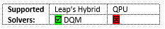
Ocean software’s dimod.DiscreteQuadraticModel contains linear and
quadratic biases for problems formulated as
discrete binary models as well as additional
information such as variable labels.
Relevant Properties#
maximum_number_of_variables defines the maximum number of problem variables.
maximum_number_of_biases defines the maximum number of problem biases.
minimum_time_limit and maximum_time_limit_hrs define the runtime duration for hybrid solvers.
Example#
This example uses Ocean software’s LeapHybridDQMSampler.
>>> from dwave.system import LeapHybridDQMSampler
>>> import dimod
>>> import random
...
>>> dqm = dimod.DiscreteQuadraticModel()
>>> for i in range(10):
...     dqm.add_variable(4)
>>> for i in range(9):
...     for j in range(i+1, 10):
...         dqm.set_quadratic_case(i, random.randrange(0, 4),
...                                j, random.randrange(0, 4), random.random())
>>> sampleset = LeapHybridDQMSampler().sample_dqm(dqm, time_limit=10)
h#
For Ising problems, the \(h\) values are the linear coefficients (biases). A problem definition comprises both h and J values.
Because the quantum annealing process minimizes the energy function of the Hamiltonian, and \(h_i\) is the coefficient of variable \(i\), returned states of the problem’s variables tend toward the opposite sign of their biases; for example, if you bias the qubits representing variable \(v_i\) with \(h_i\) values of \(-1\), variable \(v_i\) is more likely to have a final state of \(+1\) in the solution.
For QPU solvers, the programming cycle programs the solver to the specified \(h\) and \(J\) values for a given Ising problem (or derived from the specified \(Q\) values of a given QUBO problem). However, since QPU precision is limited, the \(h\) and \(J\) values realized on the solver may deviate slightly from the requested (or derived) values. For more information, see the QPU Solver Datasheet guide.
For QUBO problems, use Q instead of \(h\) and \(J\); see the Getting Started with D-Wave Solvers guide for information on converting between the formulations.
If you are submitting directly through SAPI’s REST API, see the SAPI REST Developer Guide for more information.
Default is zero linear biases.
Relevant Properties#
h_range defines the supported \(h\) range for QPU solvers.
maximum_number_of_variables defines the maximum number of problem variables for hybrid solvers.
maximum_number_of_biases defines the maximum number of problem biases for hybrid solvers.
qubits and couplers define the working graph of QPU solvers.
Interacts with Parameters#
auto_scale enables you to submit problems to QPU solvers with values outside h_range and extended_j_range and have the system automatically scale them to fit.
fast_anneal cannot be used with h values that are not zero.
Example#
This example defines a 7-qubit problem in which \(q_1\) and \(q_4\) are biased with \(-1\) and \(q_0\), \(q_2\), \(q_3\), \(q_4\), and \(q_6\) are biased with \(+1\). Qubits \(q_0\) and \(q_6\) have a ferromagnetic coupling between them with a strength of \(-1\).
>>> h = [1, -1, 1, 1, -1, 1, 1]
>>> J = {(0, 6): -1}
J#
For Ising problems, the \(J\) values are the quadratic coefficients. The larger the absolute value of \(J\), the stronger the coupling between pairs of variables (and qubits on QPU solvers). An Ising problem definition comprises both h and J values.
For QPU solvers:
This parameter sets the strength of the couplers between qubits:
\(\textbf {J < 0}\): Ferromagnetic coupling; coupled qubits tend to be in the same state, \((1,1)\) or \((-1,-1)\).
\(\textbf {J > 0}\): Antiferromagnetic coupling; coupled qubits tend to be in opposite states, \((-1,1)\) or \((1,-1)\).
\(\textbf {J = 0}\): No coupling; qubit states do not affect each other.
The programming cycle programs the solver to the specified \(h\) and \(J\) values for a given Ising problem (or derived from the specified \(Q\) values of a given QUBO problem). However, since QPU precision is limited, the \(h\) and \(J\) values realized on the solver may deviate slightly from the requested (or derived) values. For more information, see the QPU Solver Datasheet guide.
For QUBO problems, use Q instead of \(h\) and \(J\); see the Getting Started with D-Wave Solvers guide for information on converting between the formulations.
If you are submitting directly through SAPI’s REST API, see the SAPI REST Developer Guide for more information.
Default is zero quadratic biases.
Relevant Properties#
j_range defines the supported \(J\) range for QPU solvers.
extended_j_range defines an extended range of values possible for the coupling strengths for QPU solvers.
per_qubit_coupling_range defines the limits on coupling range permitted per qubit if you use extended_j_range.
maximum_number_of_variables defines the maximum number of problem variables for hybrid solvers.
maximum_number_of_biases defines the maximum number of problem biases for hybrid solvers.
qubits and couplers define the working graph of QPU solvers.
Interacts with Parameters#
auto_scale enables you to submit problems to QPU solvers with values outside h_range and extended_j_range and have the system automatically scale them to fit.
flux_biases compensates for biases introduced by strong negative couplings if you use extended_j_range.
Example#
This example defines a 7-qubit problem in which \(q_1\) and \(q_4\) are biased with \(-1\) and \(q_0\), \(q_2\), \(q_3\), \(q_4\), and \(q_6\) are biased with \(+1\). Qubits \(q_0\) and \(q_6\) have a ferromagnetic coupling between them with a strength of \(-1\).
>>> h = [1, -1, 1, 1, -1, 1, 1]
>>> J = {(0, 6): -1}
label#
Problem label you can optionally tag submissions with. You can set as a label a non-empty string of up to 1024 Windows-1252 characters that has meaning to you or is generated by your application, which can help you identify your problem submission. You can see this label on the Leap service’s dashboard and in solutions returned from SAPI.
Example#
This example submits a simple Ising problem with a label and shows how such labels are displayed on the dashboard.
>>> from dwave.system import DWaveSampler, EmbeddingComposite
>>> sampler = EmbeddingComposite(DWaveSampler())
...
>>> sampleset = sampler.sample_ising({}, {('a', 'b'): -.05},
...                                  label="Test Ising Problem 1")
>>> print(sampleset.info["problem_label"])
Test Ising Problem 1
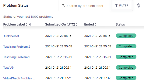
Fig. 39 Problem labels on the dashboard.#
nl#
Ocean software’s Model contains symbols
and states for problems formulated as a
nonlinear model.
Relevant Properties#
maximum_time_limit_hrs defines the maximum runtime for problems submitted to the solver.
maximum_decision_state_size defines the maximum size of all decision-variable states in a problem accepted by the solver.
maximum_number_of_nodes defines the maximum number of nodes in a problem accepted by the solver.
maximum_number_of_states defines the maximum number of initialized states in a problem accepted by the solver.
maximum_state_size defines the maximum size of all states in a problem accepted by the solver.
state_size_multiplier, num_nodes_multiplier, num_nodes_state_size_multiplier, and time_constant are used in the internal estimate of the problem’s minimum runtime.
Example#
This example creates a nonlinear model representing a flow-shop-scheduling problem with processing times for two jobs, each on three machines.
>>> from dwave.optimization.generators import flow_shop_scheduling
...
>>> processing_times = [[10, 5, 7], [20, 10, 15]]
>>> model = flow_shop_scheduling(processing_times=processing_times)
Q#
A quadratic unconstrained binary optimization (QUBO) problem is defined using an upper-triangular matrix, \(\rm \textbf{Q}\), which is an \(N \times N\) matrix of real coefficients, and \(\textbf{x}\), a vector of binary variables. The diagonal entries of \(\rm \textbf{Q}\) are the linear coefficients (analogous to \(h\), in Ising problems). The nonzero off-diagonal terms are the quadratic coefficients that define the strength of the coupling between variables (analogous to \(J\), in Ising problems).
Input may be full or sparse. Both upper- and lower-triangular values can be used; (\(i\), \(j\)) and (\(j\), \(i\)) entries are added together.
For QPU solvers
If a \(Q\) value is assigned to a coupler not present, an exception is raised. Only entries indexed by working couplers may be nonzero.
QUBO problems are converted to Ising format before they run on the solver. Ising format uses \(h\) (qubit bias) and \(J\) (coupling strength) to represent the problem; see also h and J.
The programming cycle programs the solver to the specified \(h\) and \(J\) values for a given Ising problem (or derived from the specified \(Q\) values of a given QUBO problem). However, since QPU precision is limited, the \(h\) and \(J\) values realized on the solver may deviate slightly from the requested (or derived) values. For more information, see the QPU Solver Datasheet guide.
If you are submitting directly through SAPI’s REST API, see the SAPI REST Developer Guide for more information.
Default is zero linear and quadratic biases.
Relevant Properties#
h_range and extended_j_range define the supported ranges for QPU solvers. Be aware that problems with values outside the supported range are, by default, scaled to fit within the supported range; see the auto_scale parameter for more information.
maximum_number_of_variables defines the maximum number of problem variables for hybrid solvers.
maximum_number_of_biases defines the maximum number of problem biases for hybrid solvers.
qubits and couplers define the working graph of QPU solvers.
Interacts with Parameters#
extended_j_range defines an extended range of values possible for the coupling strengths for QPU solvers.
per_qubit_coupling_range defines the limits on coupling range permitted per qubit if you use extended_j_range.
auto_scale enables you to submit problems to QPU solvers with values outside h_range and extended_j_range and have the system automatically scale them to fit.
fast_anneal cannot be used with diagonal values (linear coefficients, equivalent to h values in Ising problems) that are not zero.
Example#
This example submits a QUBO to a QPU solver.
>>> from dwave.system import DWaveSampler, EmbeddingComposite
...
>>> Q = {(0, 0): -3, (1, 1): -1, (0, 1): 2, (2, 2): -1, (0, 2): 2}
>>> sampleset = EmbeddingComposite(DWaveSampler()).sample_qubo(Q, num_reads=100)
solver#
The solver name, as a string in the JSON input data.
If you are submitting directly through SAPI’s REST API, see the SAPI REST Developer Guide for more information; Ocean software allows you to explicitly select a solver and to automatically select a solver based on your required features.
Example#
This example selects a hybrid BQM solver with binary_quadratic_model
in its name.
>>> from dwave.cloud import Client
>>> Q = {('x1', 'x2'): 1, ('x1', 'z'): -2, ('x2', 'z'): -2, ('z', 'z'): 3}
>>> with Client.from_config(solver={'name__regex': '.*binary_quadratic_model.*'}) as client:
...     solver = client.get_solver()
...     sampleset = solver.sample_qubo(Q, time_limit=5)