Solving Problems with Quantum Samplers

The What is Quantum Annealing? chapter explained how the D‑Wave QPU uses quantum annealing to find the minimum of an energy landscape defined by the biases and couplings applied to its qubits in the form of a problem Hamiltonian. As described in the Workflow: Formulation and Sampling chapter, to solve a problem by sampling, you formulate an objective function such that when the solver finds its minimum, it is finding solutions to your problem.

This chapter shows how you formulate your objective as the problem Hamiltonian of a D‑Wave quantum computer by defining the linear and quadratic coefficients of a binary quadratic model (BQM) that maps those values to the qubits and couplers of the QPU.

Binary Quadratic Models

For the QPU, two formulations for objective functions are the Ising Model and QUBO. Both these formulations are binary quadratic models and conversion between them is trivial[1].

[1]

Chapter Appendix: Next Learning Steps provides information on the differences and conversion between the two formulations.

Ising Model

The Ising model is traditionally used in statistical mechanics. Variables are “spin up” (\(\uparrow\)) and “spin down” (\(\downarrow\)), states that correspond to \(+1\) and \(-1\) values. Relationships between the spins, represented by couplings, are correlations or anti-correlations. The objective function expressed as an Ising model is as follows:

\[\text{E}_{ising}(\vc s) = \sum_{i=1}^N h_i s_i + \sum_{i=1}^N \sum_{j=i+1}^N J_{i,j} s_i s_j\]

where the linear coefficients corresponding to qubit biases are \(h_i\), and the quadratic coefficients corresponding to coupling strengths are \(J_{i,j}\).

QUBO

QUBO problems are traditionally used in computer science, with variables taking values 1 (TRUE) and 0 (FALSE).

A QUBO problem is defined using an upper-diagonal matrix \(Q\), which is an \(N\) x \(N\) upper-triangular matrix of real weights, and \(x\), a vector of binary variables, as minimizing the function

\[f(x) = \sum_{i} {Q_{i,i}}{x_i} + \sum_{i<j} {Q_{i,j}}{x_i}{x_j}\]

where the diagonal terms \(Q_{i,i}\) are the linear coefficients and the nonzero off-diagonal terms \(Q_{i,j}\) are the quadratic coefficients.

This can be expressed more concisely as

\[\min_{{x} \in {\{0,1\}^n}} {x}^{T} {Q}{x}.\]

In scalar notation, used throughout most of this document, the objective function expressed as a QUBO is as follows:

\[\text{E}_{qubo}(a_i, b_{i,j}; q_i) = \sum_{i} a_i q_i + \sum_{i<j} b_{i,j} q_i q_j.\]

Note

Quadratic unconstrained binary optimization problems—QUBOs—are unconstrained in that there are no constraints on the variables other than those expressed in Q.

Minor Embedding

A graph comprises a collection of nodes and edges, which can be used to represent an objective function’s variables and the connections between them, respectively.

For example, to represent a quadratic equation,

\[H(a,b) = 5a + 7ab - 3b,\]

you need two nodes, \(a\) and \(b\), with biases of \(5\) and \(-3\), and an edge between them with a strength of 7, as shown in Figure 29.

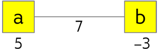
Fig. 29 Two-variable objective function.

This graphic representation means you can map a BQM representing your objective function to the QPU:

• Nodes that represent the objective function’s variables such as \(s_i\) (Ising) or \(q_i\) (QUBO) are mapped to qubits on the QPU.

• Edges that represent the objective function’s quadratic coefficients such as \(J_{i,j}\) (Ising) and \(b_{i,j}\) (QUBO) are mapped to couplers.

The process of mapping variables in the problem formulation to qubits on the QPU is known as minor embedding.

The Constraints Example: Minor-Embedding chapter demonstrates minor embedding with an example; typically Ocean software handles it automatically.

Problem-Solving Process

In summary, to solve a problem on quantum samplers, you formulate the problem as an objective function, usually in Ising or QUBO format. Low energy states of the objective function represent good solutions to the problem. Because you can represent the objective function as a graph, you can map it to the QPU:[2] linear coefficients to qubit biases and quadratic coefficients to coupler strengths. The QPU uses quantum annealing to seek the minimum of the resulting energy landscape, which corresponds to the solution of your problem.

[2]

Classical solvers might not require minor-embedding and quantum-classical hybrid solvers might embed parts of the problem on the QPU while solving other parts with classical algorithms on CPUs or GPUs.