QPU-Specific Properties

The following sections provide information for advanced users who want to better understand and leverage the physical implementation of D‑Wave’s various quantum processing units (QPUs) available in the Leap service[1]. This information includes:

• Summary of a QPU’s physical properties—The values provided are the physical properties of a calibrated QPU; they are not QPU specifications.

  Note

  In addition to the physical properties listed herein, each QPU has a number of other properties defined in software that are accessible via the Solver API. For a global list of the solver properties for a QPU, and for a list of the permitted user parameters for each type of solver, see Solver Properties and Parameters. To retrieve the solver properties for a particular QPU, see the Ocean software documentation for the syntax and examples.

• Spreadsheet for a QPU’s annealing-schedule functions and normalized annealing-waveform values—These values are required for computing the energy of a problem at a specific point in a QPU’s annealing process; as such, the spreadsheet provides the values to use for the \(A(s)\) and \(B(s)\) terms in the Hamiltonian of equation (2) for each value of the normalized anneal fraction \(s\), between 0 and 1 in increments of 0.001. Units for these terms are GHz, where the conversion from energy in Joules to Hz is through a division by Planck’s constant as follows:

  \[ \begin{align}\begin{aligned}A(s)_{\text{[GHz]}} &= \frac{A(s)_{\text{[Joules]}}} {6.62607004 \times 10^{-34} \times 10^9}\\&= 1.5092 \times 10^{24} A(s)_{\text{[Joules]}}\end{aligned}\end{align} \]

[1]

Depending on your customer contract, customer plan, and seat type in a project, you may not have access to all QPUs in the Leap service.

Advantage2_prototype2.6

All data presented in this section are specific to the Advantage2_prototype2.6 solver, which is an experimental prototype of D‑Wave’s next-generation QPU. The Advantage2™ prototype QPU is based on a physical lattice of qubits and couplers known as the Zephyr™ topology. For information, see the Zephyr Graph section in Getting Started with D-Wave Solvers.

Physical Properties

This table lists the physical properties of the calibrated QPU.

Table 37 QPU Physical Properties[2]

Property	Value
Model	\(\text{Advantage2 prototype}\)
Graph size	\(\text{Z6}\)
Number of qubits	\(1215\)
Number of couplers	\(10788\)
Qubit temperature	\(16.5 \pm 1.0\ \text{mK}\)
\(\rm M_{\rm AFM}\): Maximum mutual inductance for qubit pairs	\(0.443\ \text{pH}\)
Quantum critical point for 1D chains	\(2.014\ \text{GHz}\)
\(L_q\): Qubit inductance	\(107\ \text{pH}\)
\(C_q\): Qubit capacitance	\(207\ \text{fF}\)
\(I_c\): Qubit critical current	\(4.57\ \text{µA}\)
Average single-qubit temperature	\(0.117\)
Ferromagnetic-problem freezeout	\(0.009\)
Single-qubit freezeout	\(0.605\)
\(\Phi_{\rm CCJJ}^i\): Initial (at \(s=0\)) external flux on compound Josephson junctions	\(0.726\ \Phi_0\)
\(\Phi_{\rm CCJJ}^f\): Final (at \(s=1\)) external flux on compound Josephson junctions	\(-0.819\ \Phi_0\)
Readout time range	\(17.0\ \text{to}\ 87.0\ \text{µs}\)
Programming time	\(\sim 18200\ \text{µs}\)
QPU-delay-time per sample	\(20.5\ \text{µs}\)
Readout error rate	\(\leq 0.001\)

[2]

Some notes for the QPU properties are as follows:

• The ferromagnetic problem and single-qubit freezeout points shown are normalized anneal fraction values.

• Readout time range: Typical readout times for reading between one qubit and the full QPU.

• Programming time: Typical for problems run on this QPU. Actual problem programming times may vary slightly depending on the nature of the problem.

• Readout error rate: Error rate when reading the full system.

Annealing Schedule

Download the annealing schedule for the QPU here: Advantage2_prototype2.6 Excel spreadsheet.

The standard annealing schedule for the QPU is shown in Figure 121.

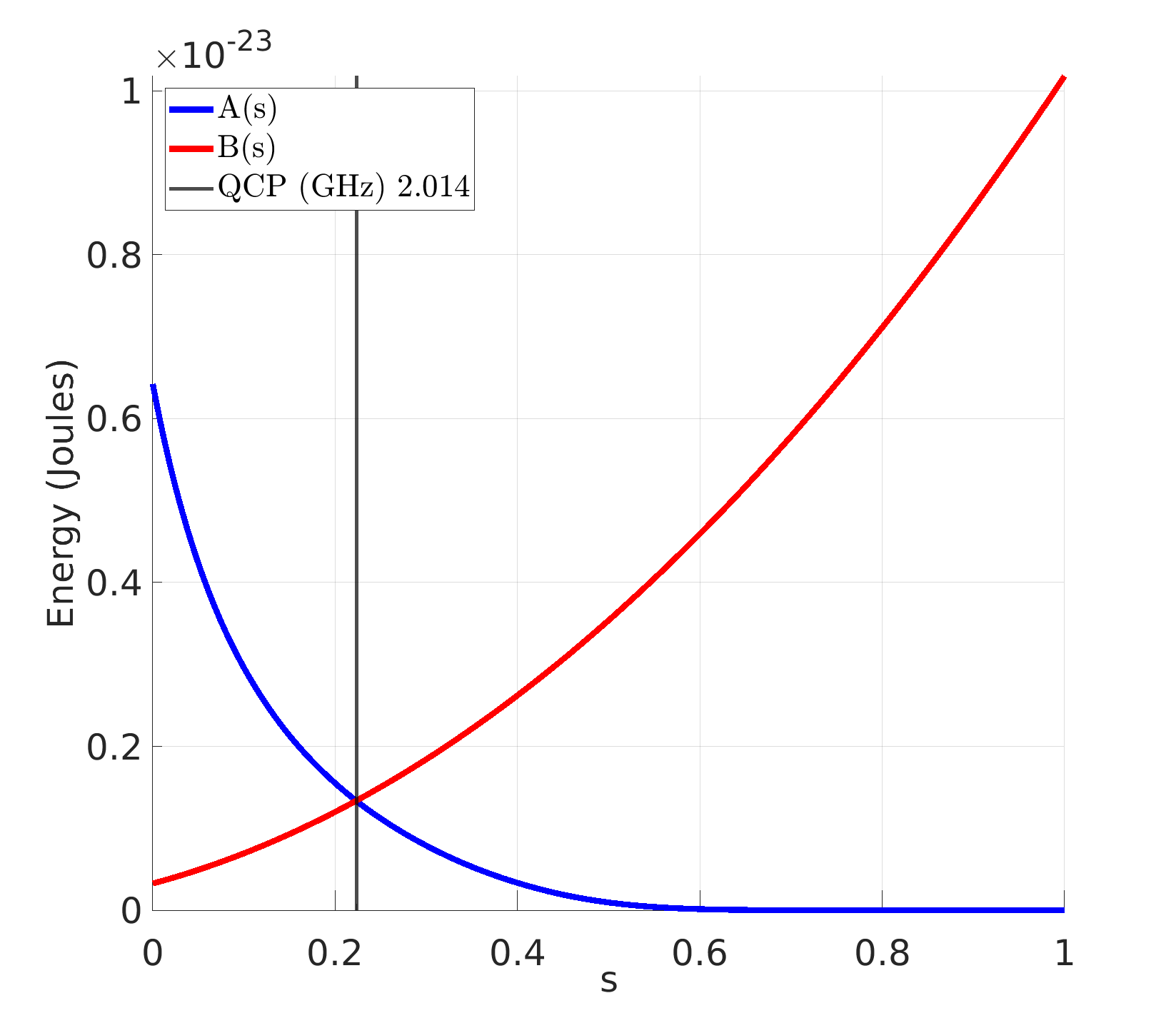
Fig. 121 Standard annealing schedule for the QPU, showing energy changes as a function of scaled time.

Advantage_system7.1

All data presented in this section are specific to the Advantage_system7.1 solver. The Advantage QPU is based on a physical lattice of qubits and couplers known as the Pegasus™ topology. For information, see the Pegasus Graph section in Getting Started with D-Wave Solvers.

Physical Properties

This table lists the physical properties of the calibrated QPU.

Table 38 QPU Physical Properties[3]

Property	Value
Model	\(\text{Advantage, performance update}\)
Graph size	\(\text{P16}\)
Number of qubits	\(5554\)
Number of couplers	\(39238\)
Qubit temperature	\(15.9 \pm 0.1\ \text{mK}\)
\(\rm M_{\rm AFM}\): Maximum mutual inductance for qubit pairs	\(1.551\ \text{pH}\)
Quantum critical point for 1D chains	\(1.277\ \text{GHz}\)
\(L_q\): Qubit inductance	\(382\ \text{pH}\)
\(C_q\): Qubit capacitance	\(123\ \text{fF}\)
\(I_c\): Qubit critical current	\(1.94\ \text{µA}\)
Average single-qubit temperature	\(0.228\)
Ferromagnetic-problem freezeout	\(0.078\)
Single-qubit freezeout	\(0.620\)
\(\Phi_{\rm CCJJ}^i\): Initial (at \(s=0\)) external flux on compound Josephson junctions	\(-0.625\ \Phi_0\)
\(\Phi_{\rm CCJJ}^f\): Final (at \(s=1\)) external flux on compound Josephson junctions	\(-0.730\ \Phi_0\)
Readout time range	\(17.0\ \text{to}\ 265.0\ \text{µs}\)
Programming time	\(\sim 17700\ \text{µs}\)
QPU-delay-time per sample	\(20.6\ \text{µs}\)
Readout error rate	\(\leq 0.001\)

[3]

Some notes for the QPU properties are as follows:

• Qubit temperature: Some qubits in this QPU are affected by high-frequency photon flux and may have a higher temperature than what is reported here. For more information, see the discussion of high-energy photon flux in QPU Solver Datasheet.

• The ferromagnetic problem and single-qubit freezeout points shown are normalized anneal fraction values.

• Readout time range: Typical readout times for reading between one qubit and the full QPU.

• Programming time: Typical for problems run on this QPU. Actual problem programming times may vary slightly depending on the nature of the problem.

• Readout error rate: Error rate when reading the full system.

Annealing Schedule

Download the annealing schedule for the QPU here: Advantage_system7.1 Excel spreadsheet.

The annealing schedule for the QPU is shown in Figure 122.

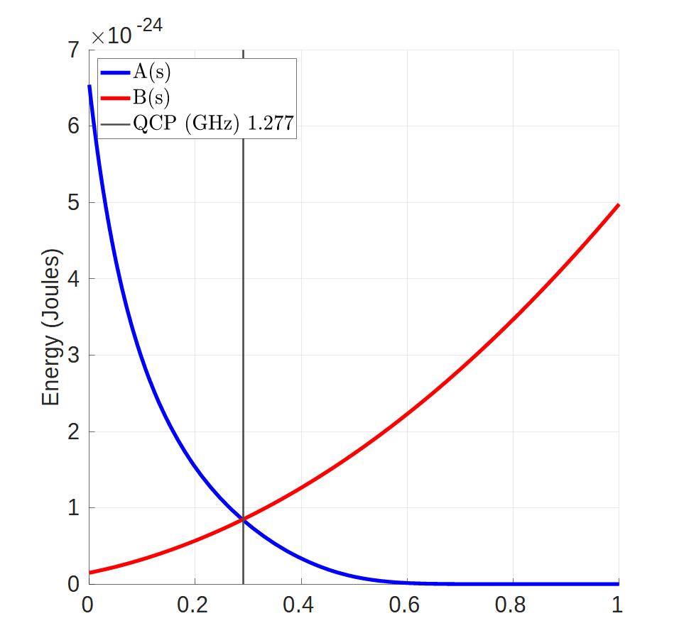
Fig. 122 Annealing schedule for the QPU, showing energy changes as a function of scaled time.

DAC Quantization Effects

The on-QPU digital-analog converters (DACs) that provide the user-specified \(h\) and \(J\) values have a finite quantization step size. That step size depends on the value of the \(h\) and \(J\) applied because the response to the DAC output is nonlinear.

Figure 123 and Figure 124 show the effects of the DAC quantization step for the DACs controlling the \(h\) and \(J\) values, respectively, for this system.

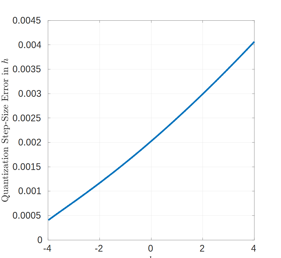
Fig. 123 Typical quantization on the \(h\) DAC control.

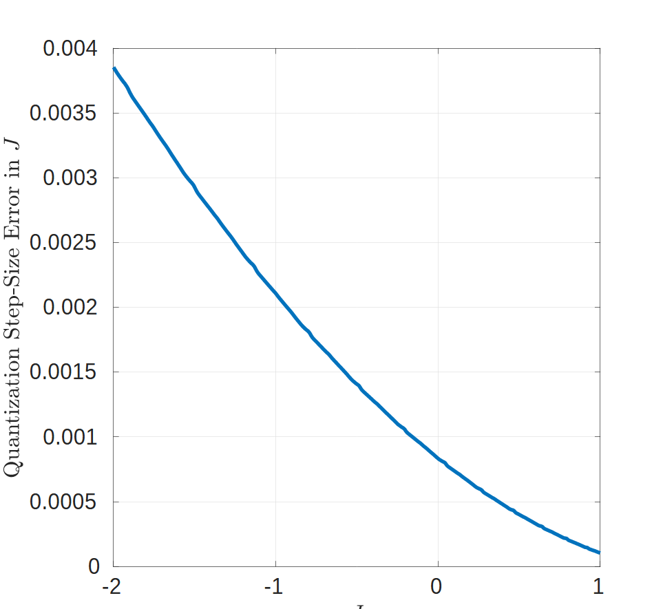
Fig. 124 Typical quantization on the \(J\) DAC control.

Advantage_system6.4

All data presented in this section are specific to the Advantage_system6.4 solver. The Advantage QPU is based on a physical lattice of qubits and couplers known as the Pegasus™ topology. For information, see the Pegasus Graph section in Getting Started with D-Wave Solvers.

Physical Characteristics

This table lists the physical properties of the calibrated QPU.

Table 39 QPU Physical Properties[4]

Property	Value
Model	\(\text{Advantage, performance update}\)
Graph size	\(\text{P16}\)
Number of qubits	\(5612\)
Number of couplers	\(40088\)
Qubit temperature	\(16.0 \pm 0.1\ \text{mK}\)
\(\rm M_{\rm AFM}\): Maximum mutual inductance for qubit pairs	\(1.554\ \text{pH}\)
Quantum critical point for 1D chains	\(1.281\ \text{GHz}\)
\(L_q\): Qubit inductance	\(382\ \text{pH}\)
\(C_q\): Qubit capacitance	\(119\ \text{fF}\)
\(I_c\): Qubit critical current	\(1.99\ \text{µA}\)
Average single-qubit temperature	\(0.221\)
Ferromagnetic-problem freezeout	\(0.073\)
Single-qubit freezeout	\(0.616\)
\(\Phi_{\rm CCJJ}^i\): Initial (at \(s=0\)) external flux on compound Josephson junctions	\(-0.624\ \Phi_0\)
\(\Phi_{\rm CCJJ}^f\): Final (at \(s=1\)) external flux on compound Josephson junctions	\(-0.723\ \Phi_0\)
Readout time range	\(18.0\ \text{to}\ 173.0\ \text{µs}\)
Programming time	\(\sim 14200\ \text{µs}\)
QPU-delay-time per sample	\(20.5\ \text{µs}\)
Readout error rate	\(\leq 0.001\)

[4]

Some notes for the QPU properties are as follows:

• Qubit temperature: Some qubits in this QPU are affected by high-frequency photon flux and may have a higher temperature than what is reported here. For more information, see the discussion of high-energy photon flux in QPU Solver Datasheet.

• The ferromagnetic problem and single-qubit freezeout points shown are normalized anneal fraction values.

• Readout time range: Typical readout times for reading between one qubit and the full QPU.

• Programming time: Typical for problems run on this QPU. Actual problem programming times may vary slightly depending on the nature of the problem.

• Readout error rate: Error rate when reading the full system.

Annealing Schedule

Download the annealing schedule for the QPU here: Advantage_system6.4 Excel spreadsheet.

The standard annealing schedule for this QPU is shown in Figure 125.

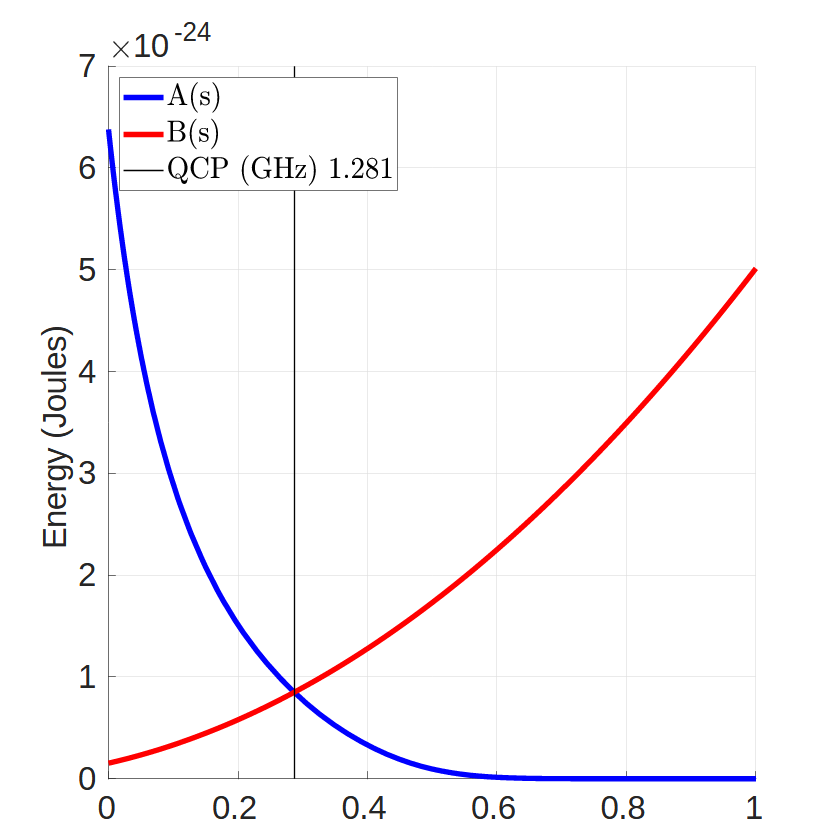
Fig. 125 Standard annealing schedule for the QPU, showing energy changes as a function of scaled time.

DAC Quantization Effects

The on-QPU digital-analog converters (DACs) that provide the user-specified \(h\) and \(J\) values have a finite quantization step size. That step size depends on the value of the \(h\) and \(J\) applied because the response to the DAC output is nonlinear.

Figure 126 and Figure 127 show the effects of the DAC quantization step for the DACs controlling the \(h\) and \(J\) values, respectively, for this system.

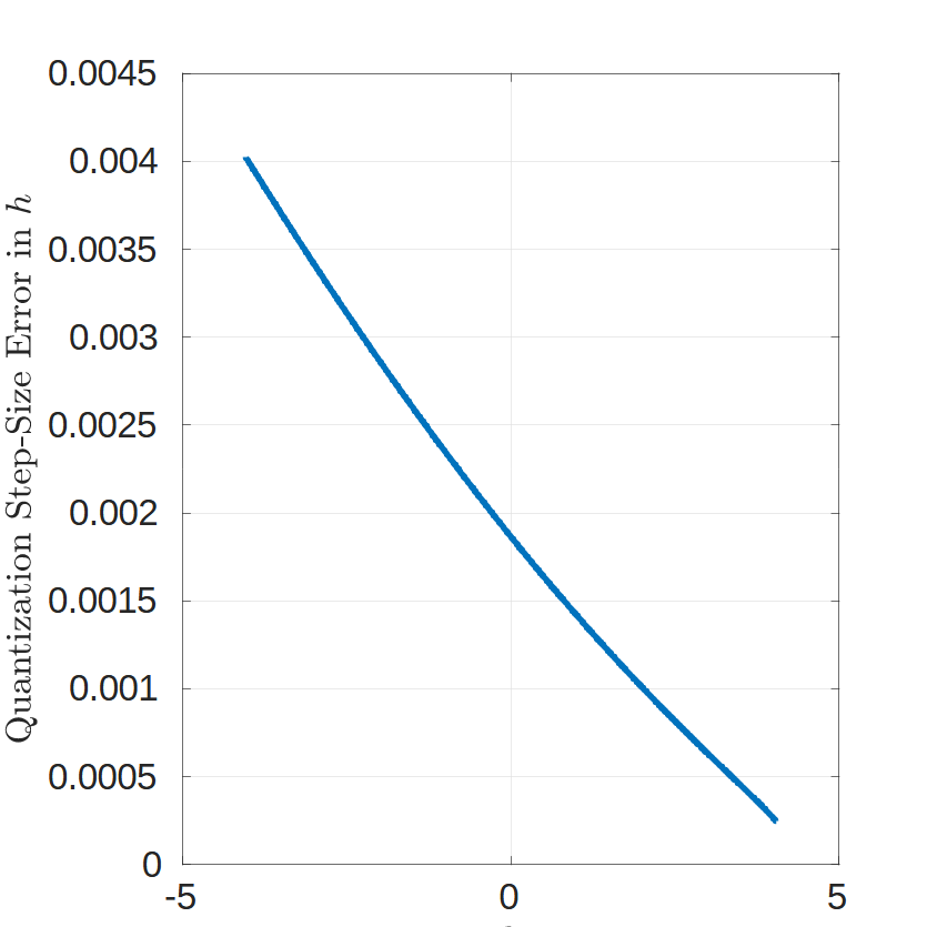
Fig. 126 Typical quantization on the \(h\) DAC control.

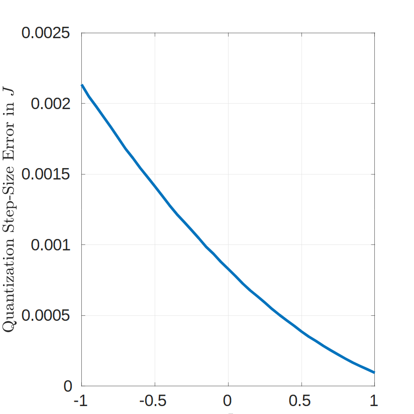
Fig. 127 Typical quantization on the \(J\) DAC control.

Advantage_system5.4

All data presented in this section are specific to the Advantage_system5.4 solver. The Advantage QPU is based on a physical lattice of qubits and couplers known as the Pegasus™ topology. For information, see the Pegasus Graph section in Getting Started with D-Wave Solvers.

Physical Characteristics

This table lists the physical properties of the calibrated QPU.

Table 40 QPU Physical Properties[5]

Property	Value
Model	\(\text{Advantage, performance update}\)
Graph size	\(\text{P16}\)
Number of qubits	\(5614\)
Number of couplers	\(40050\)
Qubit temperature	\(16.4 \pm 0.1\ \text{mK}\)
\(\rm M_{\rm AFM}\): Maximum mutual inductance for qubit pairs	\(1.687\ \text{pH}\)
Quantum critical point for 1D chains	\(1.389\ \text{GHz}\)
\(L_q\): Qubit inductance	\(375\ \text{pH}\)
\(C_q\): Qubit capacitance	\(117\ \text{fF}\)
\(I_c\): Qubit critical current	\(2.10\ \text{µA}\)
Average single-qubit temperature	\(0.193\)
Ferromagnetic-problem freezeout	\(0.067\)
Single-qubit freezeout	\(0.622\)
\(\Phi_{\rm CCJJ}^i\): Initial (at \(s=0\)) external flux on compound Josephson junctions	\(-0.620\ \Phi_0\)
\(\Phi_{\rm CCJJ}^f\): Final (at \(s=1\)) external flux on compound Josephson junctions	\(-0.714\ \Phi_0\)
Readout time range	\(18.0\ \text{to}\ 123.0\ \text{µs}\)
Programming time	\(\sim 13300\ \text{µs}\)
QPU-delay-time per sample	\(21.0\ \text{µs}\)
Readout error rate	\(\leq 0.001\)

[5]

Some notes for the QPU properties are as follows:

• Qubit temperature: Some qubits in this QPU are affected by high-frequency photon flux and may have a higher temperature than what is reported here. For more information, see the discussion of high-energy photon flux in QPU Solver Datasheet.

• The ferromagnetic problem and single-qubit freezeout points shown are normalized anneal fraction values.

• Readout time range: Typical readout times for reading between one qubit and the full QPU.

• Programming time: Typical for problems run on this QPU. Actual problem programming times may vary slightly depending on the nature of the problem.

• Readout error rate: Error rate when reading the full system.

Annealing Schedule

Download the annealing schedule for the QPU here: Advantage_system5.4.

The standard annealing schedule for the QPU is shown in Figure 128.

Fig. 128 Standard annealing schedule for the QPU, showing energy changes as a function of scaled time.

DAC Quantization Effects

The on-QPU digital-analog converters (DACs) that provide the user-specified \(h\) and \(J\) values have a finite quantization step size. That step size depends on the value of the \(h\) and \(J\) applied because the response to the DAC output is nonlinear.

Figure 129 and Figure 130 show the effects of the DAC quantization step for the DACs controlling the \(h\) and \(J\) values, respectively, for this system.

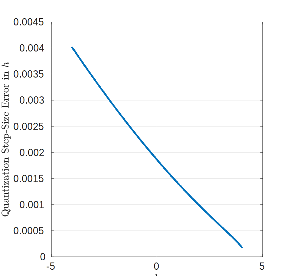
Fig. 129 Typical quantization on the \(h\) DAC control.

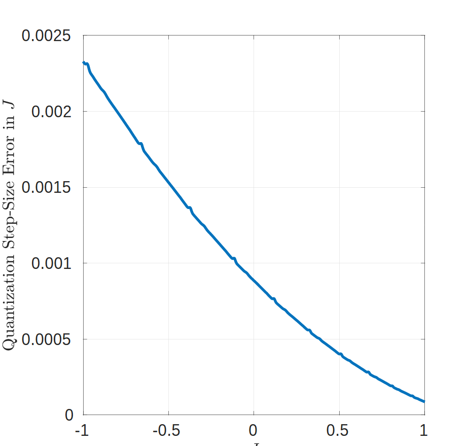
Fig. 130 Typical quantization on the \(J\) DAC control.

Advantage_system4.1

All data presented in this section are specific to the Advantage_system4.1 solver. The Advantage QPU is based on a physical lattice of qubits and couplers known as the Pegasus™ topology. For information, see the Pegasus Graph section in Getting Started with D-Wave Solvers.

Physical Properties

This table lists the physical properties of the calibrated QPU.

Table 41 QPU Physical Properties[6]

Property	Value
Model	\(\text{Advantage, performance update}\)
Graph size	\(\text{P16}\)
Number of qubits	\(5627\)
Number of couplers	\(40279\)
Qubit temperature	\(15.4 \pm 0.1\ \text{mK}\)
\(\rm M_{\rm AFM}\): Maximum mutual inductance for qubit pairs	\(1.647\ \text{pH}\)
Quantum critical point for 1D chains	\(1.391\ \text{GHz}\)
\(L_q\): Qubit inductance	\(372\ \text{pH}\)
\(C_q\): Qubit capacitance	\(119\ \text{fF}\)
\(I_c\): Qubit critical current	\(2.1\ \text{µA}\)
Average single-qubit temperature	\(0.198\)
Ferromagnetic-problem freezeout	\(0.064\)
Single-qubit freezeout	\(0.612\)
\(\Phi_{\rm CCJJ}^i\): Initial (at \(s=0\)) external flux on compound Josephson junctions	\(-0.621\ \Phi_0\)
\(\Phi_{\rm CCJJ}^f\): Final (at \(s=1\)) external flux on compound Josephson junctions	\(-0.717\ \Phi_0\)
Readout time range	\(17.0\ \text{to}\ 235.0\ \text{µs}\)
Programming time	\(\sim 14100\ \text{µs}\)
QPU-delay-time per sample	\(20.5\ \text{µs}\)
Readout error rate	\(\leq 0.001\)

[6]

Some notes for the QPU properties are as follows:

• Qubit temperature: Some qubits in this QPU are affected by high-frequency photon flux and may have a higher temperature than what is reported here. For more information, see the discussion of high-energy photon flux in QPU Solver Datasheet.

• The ferromagnetic problem and single-qubit freezeout points shown are normalized anneal fraction values.

• Readout time range: Typical readout times for reading between one qubit and the full QPU.

• Programming time: Typical for problems run on this QPU. Actual problem programming times may vary slightly depending on the nature of the problem.

• Readout error rate: Error rate when reading the full system.

Annealing Schedule

Download the annealing schedule for the QPU here: Advantage_system4.1.

The standard annealing schedule for this QPU is shown in Figure 131.

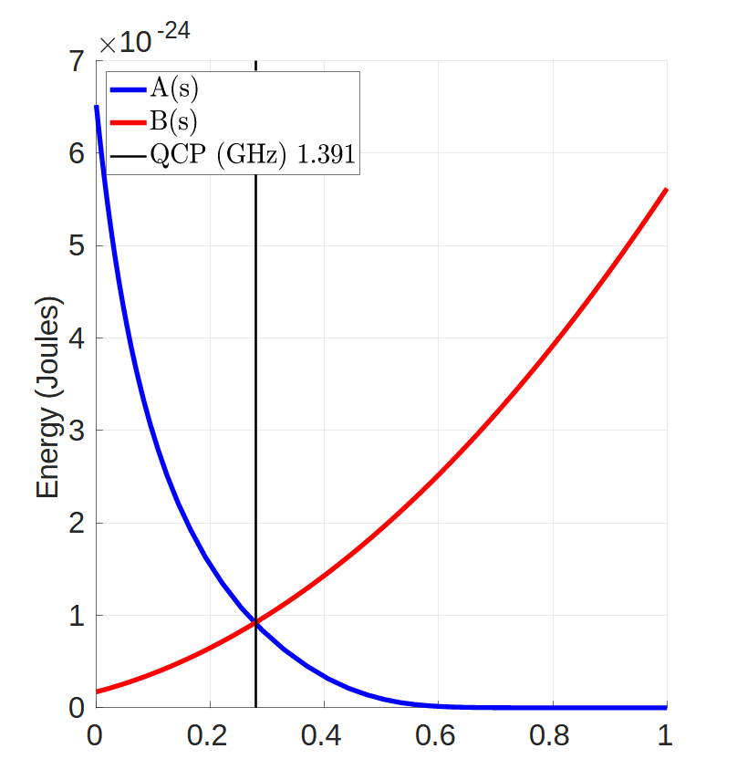
Fig. 131 Standard annealing schedule for the QPU, showing energy changes as a function of scaled time.

DAC Quantization Effects

The on-QPU digital-analog converters (DACs) that provide the user-specified \(h\) and \(J\) values have a finite quantization step size. That step size depends on the value of the \(h\) and \(J\) applied because the response to the DAC output is nonlinear.

Figure 132 and Figure 133 show the effects of the DAC quantization step for the DACs controlling the \(h\) and \(J\) values, respectively, for this system.

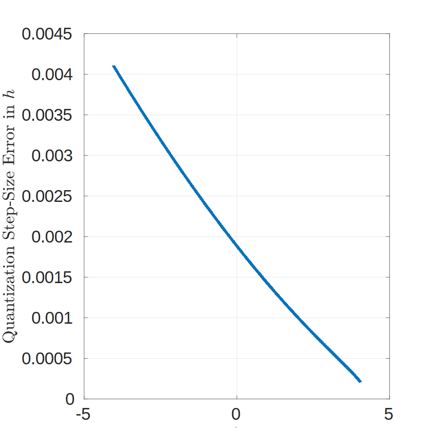
Fig. 132 Typical quantization on the \(h\) DAC control.

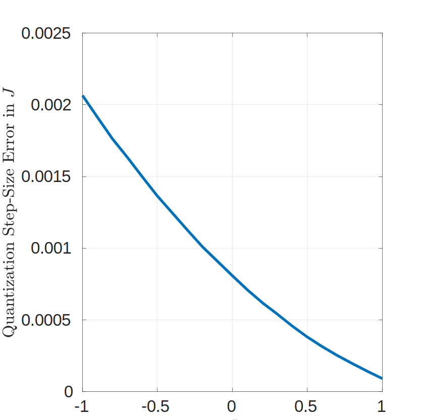
Fig. 133 Typical quantization on the \(J\) DAC control.