D‑Wave QPU Architecture: Topologies#
The layout of the D‑Wave quantum processing unit (QPU) is critical to formulating an objective function in a format that a D‑Wave annealing quantum computer can solve, as described in the Solving Problems with Quantum Samplers section. Although Ocean software automates the mapping from the linear and quadratic coefficients of a quadratic model to qubit bias and coupling values set on the QPU, you should understand it if you are using QPU solvers directly because it has implications for the problem-graph size and solution quality.
Note
If you are sending your problem to a quantum-classical hybrid solver in the Leap service, the solver handles all interactions with the QPU.
The D‑Wave QPU is a lattice of interconnected qubits. While some qubits connect to others via couplers, the D‑Wave QPU is not fully connected. Instead, the qubits of D‑Wave annealing quantum computers interconnect in one of the following topologies:
Pegasus topology for Advantage QPUs
Zephyr topology for next-generation QPUs currently under development
The Working Graph#
Some small number of qubits and couplers in a QPU may not meet the specifications to function as desired. These are therefore removed from the programmable fabric that users can access. The subset of the QPU’s graph available to users is the working graph. The yield[1] of the working graph is the percentage of working qubits that are present.
Topology Concepts and the Chimera Topology#
This section introduces concepts in topology by describing elements of the Chimera™ topology used on D‑Wave’s previous generation of quantum computer, the D‑Wave 2000Q™ system. The Chimera topology’s relative simplicity is helpful for understanding the more complex topologies of newer QPUs: in addition to shared concepts, the newer topologies are often described in terms derived from the Chimera topology.
Qubit Orientation#
Qubits on D‑Wave QPUs are “oriented” vertically or horizontally as shown in Figure 12 for the Chimera topology.

Fig. 12 Qubits represented as horizontal and vertical loops. This graphic shows three rows of 12 vertical qubits and three columns of 12 horizontal qubits for a total of 72 qubits, 36 vertical and 36 horizontal.#
Qubits on newer QPUs, such as those with the Zephyr topology, are also oriented vertically and horizontally.
Coupler Types#
It is conceptually useful to categorize couplers as follows:
Internal couplers.
Internal couplers connect pairs of orthogonal (with opposite orientation) qubits as shown in Figure 13.
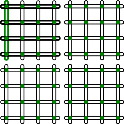
Fig. 13 Green circles at the intersections of qubits signify internal couplers; for example, the upper leftmost vertical qubit, highlighted in green, internally couples to four horizontal qubits, shown bolded.#
External couplers.
External couplers connect colinear pairs of qubits—pairs of parallel qubits in the same row or column—as shown in Figure 14.
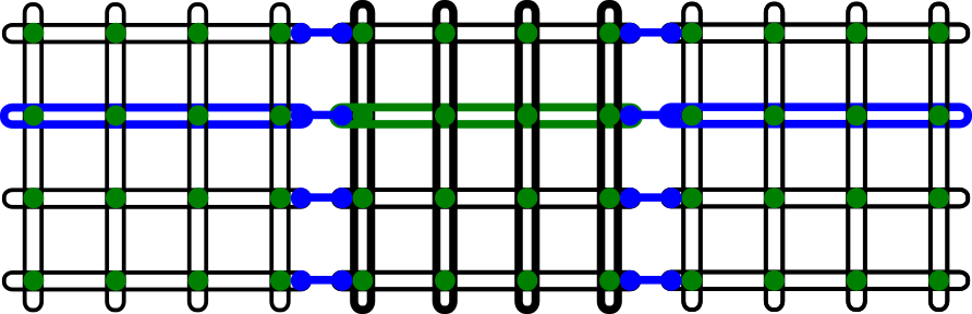
Fig. 14 External couplers, shown as connected blue circles, couple vertical qubits to adjacent vertical qubits and horizontal qubits to adjacent horizontal qubits; for example, the green horizontal qubit in the center couples to the two blue horizontal qubits in adjacent unit cells. (It is also coupled to the bolded qubits in its own unit cell by internal couplers.)#
Odd couplers.
Odd couplers connect similarly aligned pairs of qubits as shown in Figure 23 of the Pegasus Graph section. The Chimera topology does not support such couplers but newer topologies do.
Unit Cells#
The Chimera topology has a recurring structure of four horizontal qubits coupled to four vertical qubits in a \(K_{4,4}\) bipartite graph, called a unit cell. Figure 15 shows three unit cells.
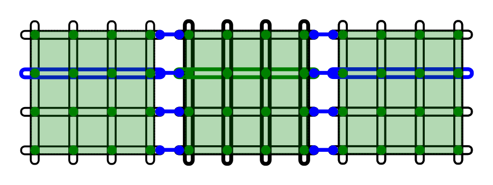
Fig. 15 Three unit cells in the Chimera topology. Each of the three green squares contains eight qubits, four horizontal and four vertical. External couplers couple horizontal qubits to adjacent horizontal qubits (shown as connected blue circles) and vertical qubits to adjacent vertical qubits (not shown). Internal couplers, shown in green, couple horizontal to vertical qubits inside each unit cell.#
A unit cell is typically rendered as either a cross or a column as shown in Figure 16.
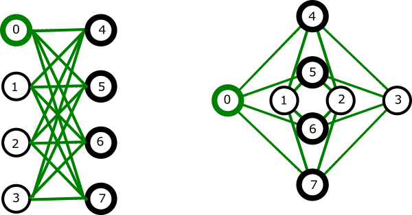
Fig. 16 Unit cell in the Chimera topology. In each of these renderings there are two sets of four qubits. Each qubit connects to all qubits in the other set but to none in its own, forming a \(K_{4,4}\) graph; for example, the green qubit labeled 0 connects to bolded qubits 4 to 7.#
Structure#
The \(K_{4,4}\) unit cells formed by internal couplers are connected by external couplers as a lattice: this is the Chimera topology. Figure 17 shows two unit cells that form part of a larger Chimera graph.
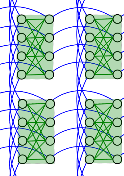
Fig. 17 A cropped view of two unit cells of a Chimera graph. Qubits are arranged in 4 unit cells (translucent green squares) interconnected by external couplers (blue lines).#
Notations#
Qubits in the Chimera topology are characterized as having:
nominal length 4—each qubit is connected to 4 orthogonal qubits through internal couplers
degree 6—each qubit is coupled to 6 different qubits
The notation CN refers to a Chimera graph consisting of an \(N{\rm x}N\) grid of unit cells.
For example, the D‑Wave 2000Q QPU supported a C16 Chimera graph: its more than 2000 qubits were logically mapped into a \(16 {\rm x} 16\) matrix of unit cells of 8 qubits. The \(2 {\rm x} 2\) Chimera graph of Figure 13 is denoted C2.
Pegasus Graph#
In Advantage™ QPUs, qubits are “oriented” vertically or horizontally, as in the Chimera topology, but similarly aligned qubits are also shifted, as illustrated in Figure 18.

Fig. 18 A cropped view of the Pegasus topology with qubits represented as horizontal and vertical loops. This graphic shows approximately three rows of 12 vertical qubits and three columns of 12 horizontal qubits for a total of 72 qubits, 36 vertical and 36 horizontal.#
For QPUs with the Pegasus™ topology it is conceptually useful to categorize couplers as internal, external, and odd. Figure 19 and Figure 20 show two views of the coupling of qubits in this topology.
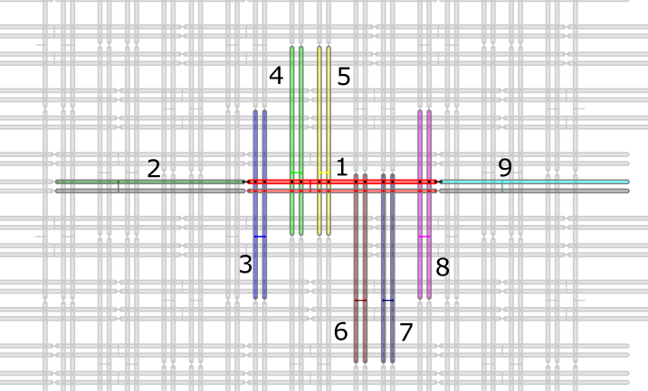
Fig. 19 Coupled qubits (represented as horizontal and vertical loops): the horizontal qubit in the center, shown in red and numbered 1, with its odd coupler and paired qubit also in red, is internally coupled to vertical qubits, in pairs 3 through 8, each pair and its odd coupler shown in a different color, and externally coupled to horizontal qubits 2 and 9, each shown in a different color.#
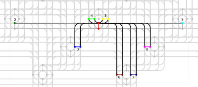
Fig. 20 Coupled qubits “roadway” graphic (qubits represented as dots and couplers as lines): the qubit in the upper center, shown in red and numbered 1, is oddly coupled to the (red) qubit shown directly below it, internally coupled to vertical qubits, in pairs 3 through 8, each pair and its odd coupler shown in a different color, and externally coupled to horizontal qubits 2 and 9, each shown in a different color.#
Couplers#
Internal couplers.
Internal couplers connect pairs of orthogonal (with opposite orientation) qubits as shown in Figure 21. Each qubit is connected via internal coupling to 12 other qubits.

Fig. 21 Junctions of horizontal and vertical loops signify internal couplers; for example, the green vertical qubit is coupled to 12 horizontal qubits, shown bolded. The translucent green square represents a unit cell structure in the Chimera topology (a \(K_{4,4}\) bipartite graph of internal couplings).#
External couplers.
External couplers connect vertical qubits to adjacent vertical qubits and horizontal qubits to adjacent horizontal qubits as shown in Figure 22.
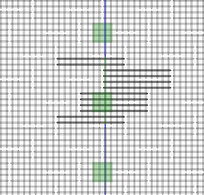
Fig. 22 External couplers connect similarly aligned adjacent qubits; for example, the green vertical qubit is coupled to the two adjacent vertical qubits, highlighted in blue.#
Odd couplers.
Odd couplers connect similarly aligned pairs of qubits as shown in Figure 23.
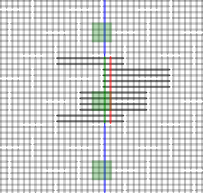
Fig. 23 Odd couplers connect similarly aligned pairs of qubits; for example, the green vertical qubit is coupled to the red vertical qubit by an odd coupler.#
The Pegasus topology features qubits of degree 15 and native \(K_4\) and \(K_{6,6}\) subgraphs. Qubits in this topology are considered to have a nominal length of 12 (each qubit is connected to 12 orthogonal qubits through internal couplers) and degree of 15 (each qubit is coupled to 15 different qubits).
As the notation \(C_n\) refers to a Chimera graph with size parameter N, \(P_n\) refers to instances of Pegasus topologies; for example, \(P_3\) is a graph with 144 nodes. A unit cell in the Pegasus topology contains twenty-four qubits, with each qubit coupled to one similarly aligned qubit in the cell and two similarly aligned qubits in adjacent cells, as shown in Figure 24. An Advantage QPU is a lattice of \(16x16\) such unit cells, denoted as a \(P_{16}\) Pegasus graph.
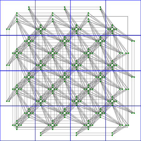
Fig. 24 Unit cells of the Pegasus topology in a \(P_4\) graph, with qubits represented as green dots and couplers as gray lines.#
More formally, a unit cell in the Pegasus topology consists of 48 halves of qubits that are divided between adjacent such unit cells, as shown in Figure 25.
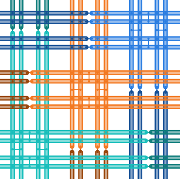
Fig. 25 Unit cell in the Pegasus topology shown as 48 halves of qubits from adjacent unit cells, with qubits represented as truncated loops (double lines), internal couplers as dots, and external and odd couplers as dots connected by short lines.#
Zephyr Graph#
D‑Wave is currently developing its next-generation QPU with the Zephyr™ topology: qubits are “oriented” vertically or horizontally, as in the Chimera and Pegasus topologies, and are shifted and connected with three coupler types as in the Pegasus topology, but this new graph achieves higher nominal length (16) and degree (20). A qubit in the Zephyr topology has sixteen internal couplers connecting it to orthogonal qubits and two external couplers and two odd couplers connecting it to similarly aligned qubits.
The Zephyr topology enables native \(K_4\) and \(K_{8,8}\) subgraphs.
Figure 26 shows the 20 couplers of a qubit in a Zephyr graph.
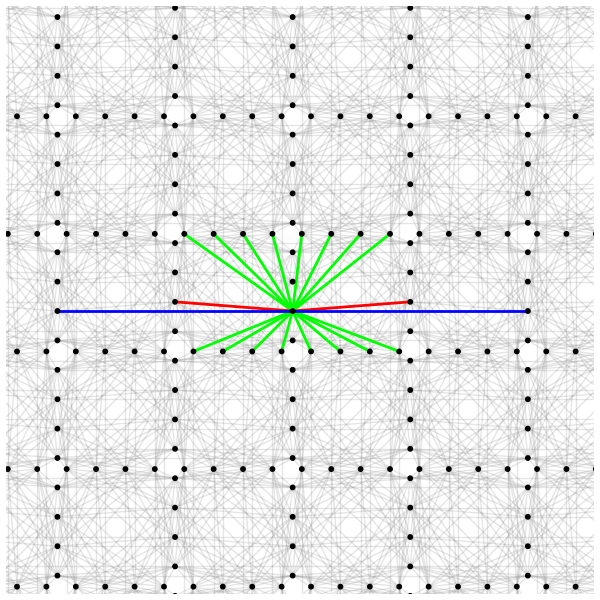
Fig. 26 A cropped view of the Zephyr topology with one representative qubit (black dot) connected to orthogonal qubits by 16 internal couplers (green lines) and to similarly aligned qubits by two external couplers (blue lines) and two odd couplers (red lines).#
As the notations \(C_n\) and \(P_n\) refer to Chimera and Pegasus graphs with size parameter N, \(Z_n\) refers to instances of Zephyr topologies; specifically, \(Z_n\) is a \((2n+1) \times (2n+1)\) grid of unit cells. For example, \(Z_3\) is a graph with 336 nodes.
As shown in Figure 27, a unit cell in the Zephyr topology contains two groups of eight half qubits, with each qubit in the cell coupled either to four oppositely aligned qubits and one similarly aligned qubit (four \(K_{4,4}\) complete graphs with their internal and external couplings) or to eight oppositely aligned qubits and one similarly aligned qubit (a \(K_{8,8}\) complete graph with its internal and odd couplings).
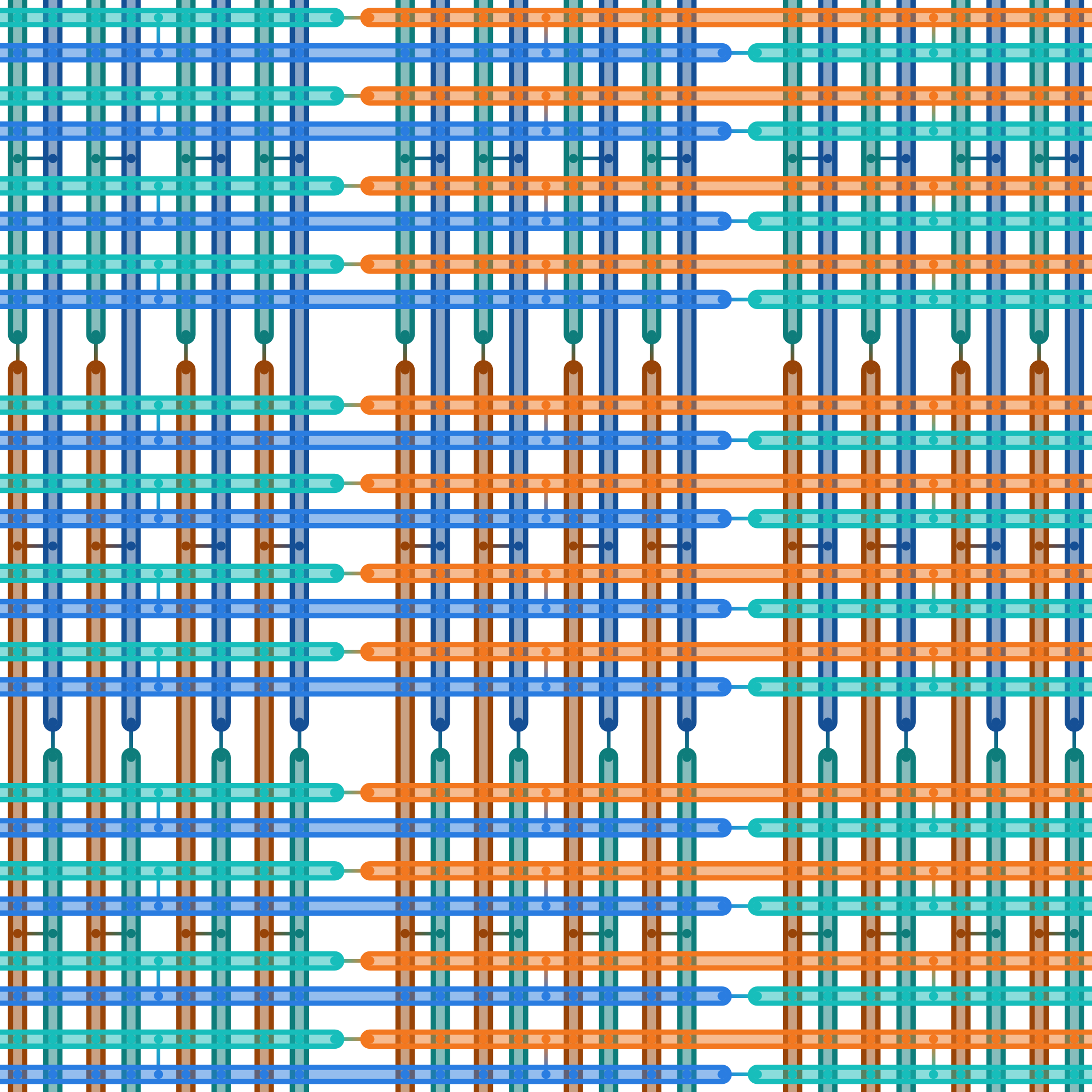
Fig. 27 Unit cells in the Zephyr topology: for the center unit cell, one group of eight half qubits are shown in orange, another in blue.#
Figure 28 shows a \(Z_1\) \(3X3\) grid of unit cells in the Zephyr topology.
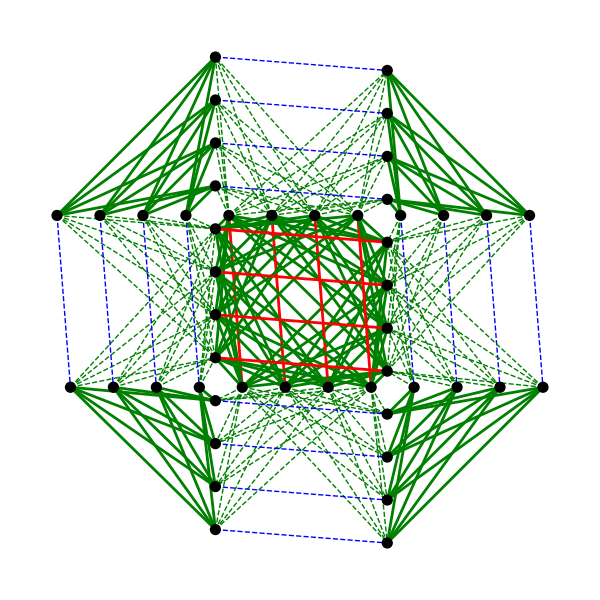
Fig. 28 A visualization of the \(Z_1\) \(3X3\) grid of unit cells in the Zephyr topology: qubits are represented as black dots, solid lines represent couplers that belong to one unit cell, while dashed lines represent couplers that belong to other unit cells. Internal couplers are green, external couplers are blue, and odd coupler are red.#
Ocean Software’s Graph Tools#
Ocean software provides for all supported topologies the following graph tools:
graph generation creates graphs for the supported topologies of various sizes.
drawing visualizes the graphs you create.
indexing helps translate coordinates of the supported graphs.
Further Information: Technical Reports#
You can learn more about these topologies and their implications in the following technical reports:
Pegasus topology: 14-1026 Next-Generation Topology of D-Wave Quantum Processors
Zephyr topology: 14-1056 Zephyr Topology of D-Wave Quantum Processors