Annealing Implementation and Controls#
This section describes how quantum annealing (QA) is implemented and features that allow you to control the annealing process[1].
Per-qubit anneal offsets: adjust the standard annealing path per qubit.
Global anneal schedule: enable mid-anneal quench and pause, reverse annealing, and fast annealing.
QA Implementation#
The superconducting QPU at the heart of the D‑Wave system, which operates at a temperature below 20 mK, is a controllable, physical realization of the quantum Ising spin system in a transverse field. Each qubit and coupler on the QPU has several controls that are manipulated by individual on-QPU digital-to-analog converters (DACs); see [Bun2014] and [Joh2010]. Along with the DACs, a small number of analog control lines provide the time-dependent control required by the quantum Hamiltonian:
where \({\hat\sigma_{x,z}^{(i)}}\) are Pauli matrices operating on a qubit \(q_i\) (the quantum one-dimensional Ising spin), and nonzero values of \(h_i\) and \(J_{i,j}\) are limited to those available in the QPU graph; see the QPU Architecture section of the Getting Started with D-Wave Solvers guide.
The quantum annealing process occurs between time \(t=0\) and time \(t_f\), which users specify via the annealing_time parameter or according to a schedule set with the anneal_schedule parameter. For simplicity, this is parameterized as \(s\), the normalized anneal fraction, which ranges from 0 to 1.
At time \(t=0\) (\(s=0\)), \(A(0) \gg B(0)\), which leads to a trivial and easily initialized quantum ground state of the system where each spin, \(s_i\), is in a delocalized combination of its classical states \(s_i = \pm 1\). The system is then annealed by decreasing \(A\) and increasing \(B\) until time \(t_f\) (\(s=1\)), when \(A(1) \ll B(1)\), and the qubits have dephased to classical systems and the \({\hat\sigma_{z}^{(i)}}\) can be replaced by classical spin variables \(s_i = \pm 1\). At this point, the system is described by the classical Ising spin system
such that the classical spin states represent a low-energy solution.
Figure 81 shows how \(A\) and \(B\) change over time for a standard anneal.
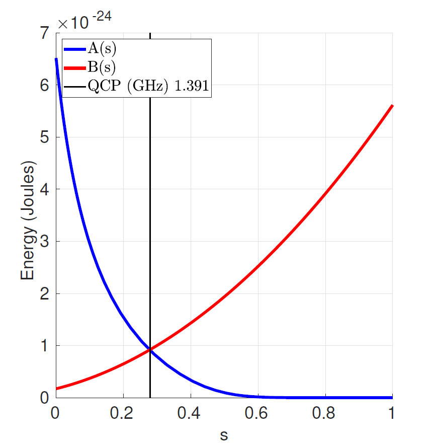
Fig. 81 Annealing functions \(A(s)\), \(B(s)\). Annealing begins at \(s=0\) with \(A(s) \gg B(s)\) and ends at \(s=1\) with \(A(s) \ll B(s)\). The quantum critical point (QCP) is the point in the anneal where the amplitudes of \(A(s)\) and \(B(s)\) are equal. Data shown are representative of Advantage™ systems.#
Hardware: Coupled Flux Qubits#
The D‑Wave QPU is a network of calibrated, superconducting flux qubits that are tunably coupled; see [Har2010_2]. The physical Hamiltonian of this set of flux qubits in the qubit approximation is
where \(\Delta_q\) is the energy difference between the two eigenstates of the qubit with no external applied flux (the degeneracy point) where the eigenstates are \((\ket{0} \pm \ket{1})/\sqrt{2}\). This energy difference captures the contribution of coherent tunneling between the two wells. \(I_p\) represents the magnitude of the current flowing in the body of the qubit loop; see Figure 82. \(M_{\rm AFM}\) is the maximum mutual inductance generated by the couplers between the qubits (typically 2 pH), \(\Phi_i^x(s)\) is an external flux applied to the qubits, and \(\Phi_{\rm CCJJ}(s)\) is an external flux applied to every qubit’s compound Josephson-junction structures to change the potential energy shape of the qubit.
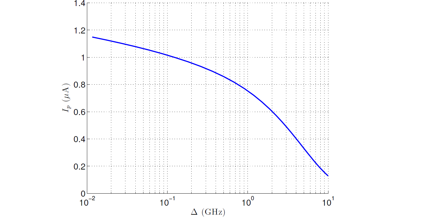
Fig. 82 Typical \(I_p\) vs \(\Delta_q\). This relationship is fixed by the physical parameters of the flux qubit. Data shown are representative of D‑Wave 2X systems.#
The relationship between \(\Delta_q(\Phi_{\rm CCJJ})\) and \(I_p(\Phi_{\rm CCJJ})\) is fixed by the physical parameters of the flux qubit. Changing the applied \(\Phi_{\rm CCJJ}\) moves the flux qubit along the curve shown in Figure 82.
Standard-Anneal Protocol#
To map the QPU’s Hamiltonian to equation (2), set \(\Phi^x_i(s) = M_{\rm AFM} |I_p(s)|\). Thus, as \(\Phi_{\rm CCJJ}(s)\) changes during the anneal, \(\Phi^x_i(s)\) changes as required to keep the relative energy ratio between the \(h\) and \(J\) terms constant. In particular, the physical flux applied to the qubit to implement a fixed \(h\) value increases as the anneal progresses. Then, the mapping to the Ising Hamiltonian becomes:
For simplicity, introduce a normalized annealing bias,
where \(\Phi_{\rm CCJJ}^{\rm initial}\) and \(\Phi_{\rm CCJJ}^{\rm final}\) are the values of \(\Phi_{\rm CCJJ}\) at \(s = 0\) and \(s = 1\), respectively (\(c(0) = 0\) and \(c(1)\) = 1).
The signal \(c(s)\) is provided by an external room-temperature current source. The time-dependence of this bias signal is chosen to produce a linear growth in time of the persistent current flowing in the qubits, \(I_p(s)\). Because \(B(s) = 2 M_{\rm AFM} I_p(s)^2\), the problem energy scale grows quadratically in time (as seen in Figure 81).
Fast-Anneal Protocol#
Depending on the length of time chosen for the quantum annealing process to execute (i.e., \(t_f\)), one can distinguish between three regimes (see [Ami2015]) of the quantum dynamics:
Coherent: the anneal is too fast to be much affected by the environment (the QPU acts as though it were a closed system).
Non-equilibrium: the anneal is slow enough for the environment to start to cause the system to occupy excited states, but not slow enough to establish thermal equilibrium.
Quasistatic: the anneal is so slow that the system follows equilibrium during most of the evolution.
Some QPUs support an alternate anneal protocol, fast anneal, that enables you to execute an anneal within the coherent regime; for example, \(0 \le t \le t_f=7~\text{ns}\). This is the anneal protocol used in experiments such as [Kin2022].
In this protocol, instead of shaping the signal from the external current source, \(c(s)\), to produce a linear growth of the qubits’ persistent current, \(I_p(s)\), the flux applied to all qubits, \(\Phi_{\rm CCJJ}(s)\), is ramped up linearly. This enables the QPU to complete an anneal in mere nanoseconds, well within the coherent regime.
However, for these potentially very fast ramps in \(\Phi_{\rm CCJJ}(s)\), no attempt is made to keep the relative energy ratio between \(h\) and \(J\) terms constant (through adjustments of \(\Phi^x_i(s)\), as is done by the standard-anneal protocol, where it is set to the linear \(M_{\rm AFM} |I_p(s)|\)). Consequently, this protocol is used only for problems with no linear biases (\(h=0\)).
Note
Although linear biases must be zero when using the fast-anneal protocol, for some problems you can emulate these biases by coupling a problem qubit to an ancillary qubit to which a flux-bias offset is applied.
See an example in the D-Wave Problem-Solving Handbook.
Energy Scales#
Energy scales \(A(s)\) and \(B(s)\) can be described, based on the parameters defined in the Hardware: Coupled Flux Qubits section above, as follows:
\(A(s)\) represents the transverse, or tunneling, energy. It equals \(\Delta_q\), the energy difference between the two eigenstates of the qubit with no external applied flux.
\(B(s)\) is the energy applied to the problem Hamiltonian. It equals \(2M_{\rm AFM}I_p(s)^2\), where \(M_{\rm AFM}\) represents the maximum available mutual inductance achievable between pairs of flux qubit bodies and \(I_p\) is the magnitude of the current flowing in the body of the qubit loop.
A single, global, time-dependent bias controls the changes of energy scales \(A(s)\) and \(B(s)\) during the quantum annealing process. At any intermediate value of \(s\), the ratio \(A(s)/B(s)\) is fixed. You can choose the trajectory of one of \(A\) or \(B\) with time.
For the standard-annealing protocol, where \(I_p(s)\) grows linearly with time, \(B(s)\) grows quadratically. Typical values of \(A(s)\) and \(B(s)\) are shown in Figure 81.
For the fast-anneal protocol, where \(\Phi_{\rm CCJJ}(s)\) increases linearly with time, \(A(s)\) and \(B(s)\) are produced by the linear growth of the signal \(c(s)\) . A typical plot of \(A(c(s))\) and \(B(c(s))\) is shown in Figure 83.
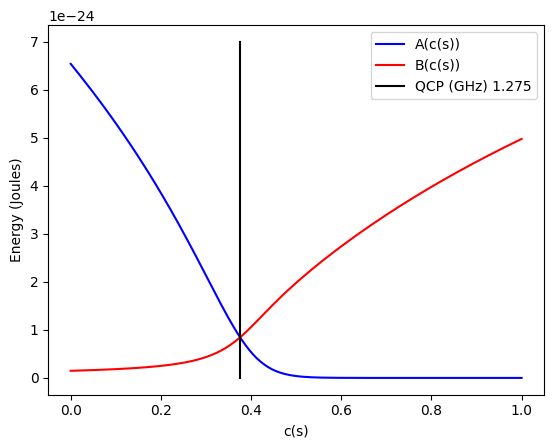
Fig. 83 Annealing functions \(A(c(s))\) and \(B(c(s))\) for fast anneal. Data shown are representative of Advantage systems.#
Note
If you are using the Leap quantum cloud service from D‑Wave, you can find the \(A(s)\) and \(B(s)\) and \(c(s)\) values for the QPUs here: QPU-Specific Characteristics. If you have an on-premises system, contact D‑Wave to obtain the values for your system.
Freezeout Points#
\(A(s)\) sets the time scale for qubit dynamics. As annealing progresses, \(A(s)\), and therefore this time scale, decreases. When the dynamics of the complex Ising spin system become slow compared to \(t_f\), the network is frozen—that is, the spin state does not change appreciably as the Ising spin Hamiltonian evolves. While in general each Ising spin problem has different dynamics, it is instructive to analyze a simple system consisting of clusters of uniformly coupled qubits. These clusters of coupled qubits are called logical qubits.[2]
Networks of logical qubits freeze out at different points in the annealing process, depending on several factors, including:
Number of qubits in the network
Coupling strengths between the qubits
Overall time scale of the anneal, \(t_f\)
In general, freezeout points move earlier in \(s\) for larger logical qubit sizes, for more strongly coupled logical qubits, and for smaller annealing time \(t_f\). Figure 84 and Figure 85 show representative freezeout points for several qubit network sizes. A network of logical qubits is created by coupling multiple qubits to a single central qubit using \(J = +1\); see the Using Two-Spin Systems to Measure ICE section for more details.
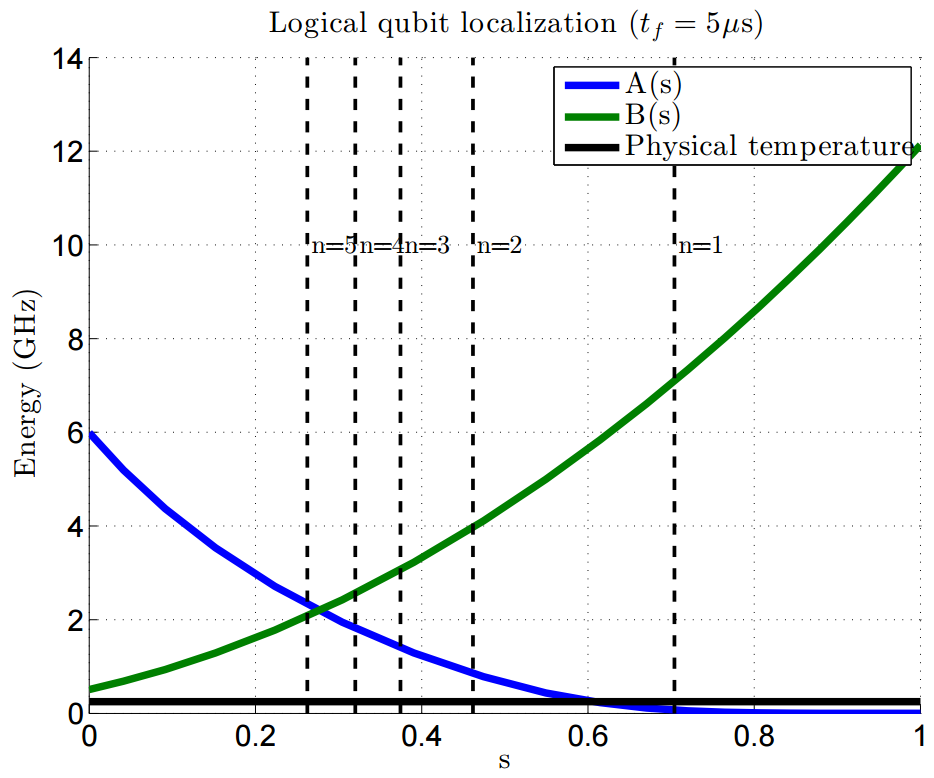
Fig. 84 Representative annealing schedules with freezeout points for several logical qubit sizes and \(t_f = 5\ \mu s\). The dashed lines show localization points for a \(N = 1\) through \(N = 5\) logical qubit clusters from right to left, respectively. Data shown are representative of D‑Wave 2X systems.#
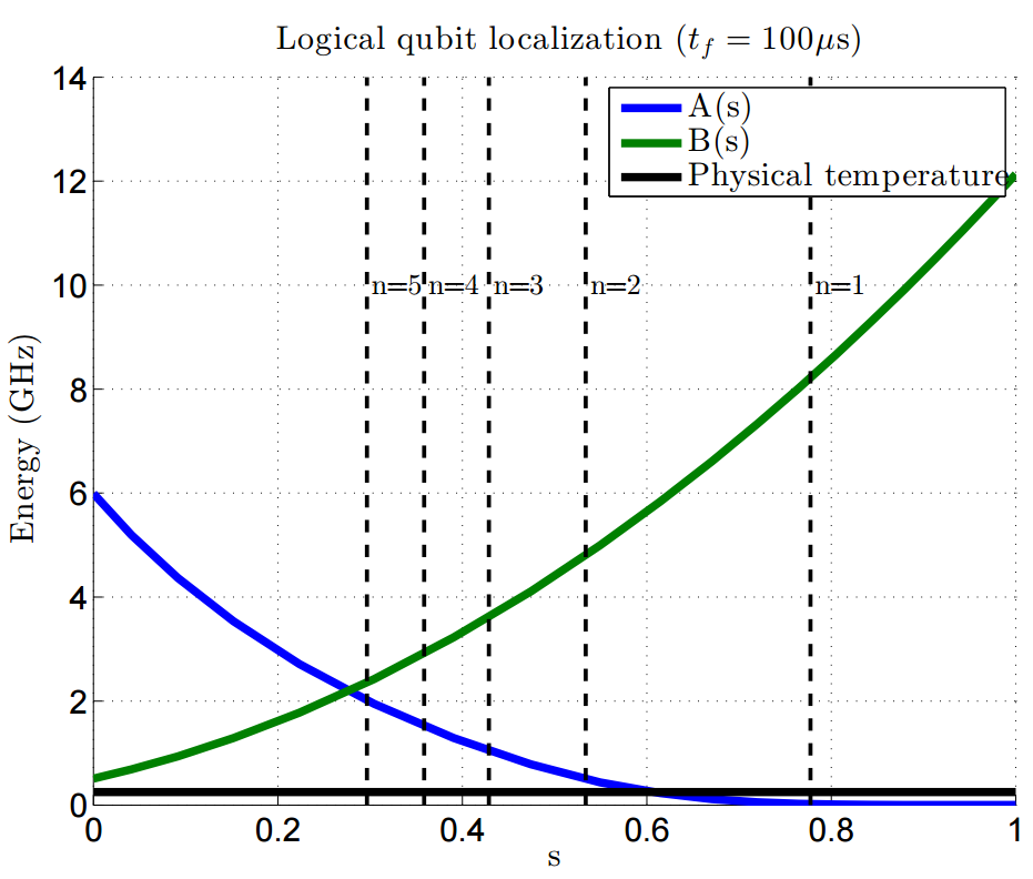
Fig. 85 Representative annealing schedules with freezeout points for several logical qubit sizes and \(t_f = 100\ \mu s\). The dashed lines show localization points for a \(N = 1\) through \(N = 5\) logical qubit clusters from right to left, respectively. Data shown are representative of D‑Wave 2X systems.#
Measuring[3] \(I_p\) at the freezeout point of various-sized logical qubits results in Figure 86. The figure shows that less annealing time and larger clusters move the freezeout point earlier in the anneal, where \(I_p\) is lower.
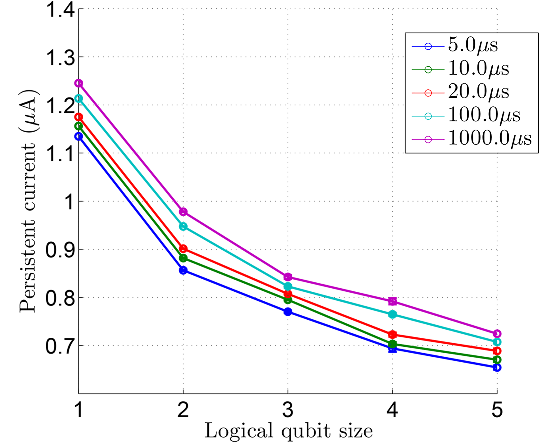
Fig. 86 \(I_p\) (persistent current) at the freezeout point as a function of logical qubit size and annealing time. The change in \(I_p\) at freezeout, as the annealing time varies from 5 to 1000 \(\mu s\) and the logical spin cluster size varies from 1 to 5. Shorter annealing time and larger clusters move the freezeout point earlier in the anneal, where \(I_p\) is lower. Data shown are representative of D‑Wave 2X systems.#
The signal corresponding to fixed \(h\) values scales as \(I_p\). Larger logical qubits freeze out earlier in the annealing process: at lower \(I_p\). Thus, if an erroneous fixed flux offset exists in the physical body (a static addition to the term \(\Phi^x_i\)), then the corresponding \(\delta h\) at freezeout grows with the logical qubit size because of the lower persistent current at the freezeout point. This error should roughly double going from a logical qubit of size 1 to a logical qubit of size 5. The standard deviation of \(\delta h\) versus logical qubit size plot in Figure 96 indicates that this is approximately true.
Anneal Offsets#
The standard annealing trajectory lowers \(A(s)\) and raises \(B(s)\) identically for all qubits in the QPU. This single annealing path, however, may not be ideal for some applications of quantum annealing. This section describes anneal offsets, which allow you to adjust the standard annealing path per qubit.
As discussed above, the annealing process is controlled via a global, time-dependent bias signal \(c(s)\) that simultaneously modifies both \(A(s)\) and \(B(s)\). Figure 81 shows typical \(A(s)\) and \(B(s)\) across the annealing algorithm; values of \(A(s)\), \(B(s)\), and \(c(s)\) for QPUs can be found on the QPU-Specific Characteristics page. Figure 87 plots the annealing bias \(c(s)\) versus \(s\). Because of the shape of the qubit energy potential, \(c(s)\) is not linear in \(s\) but is chosen to ensure that \(I_p(s)\) grows linearly with \(s\).
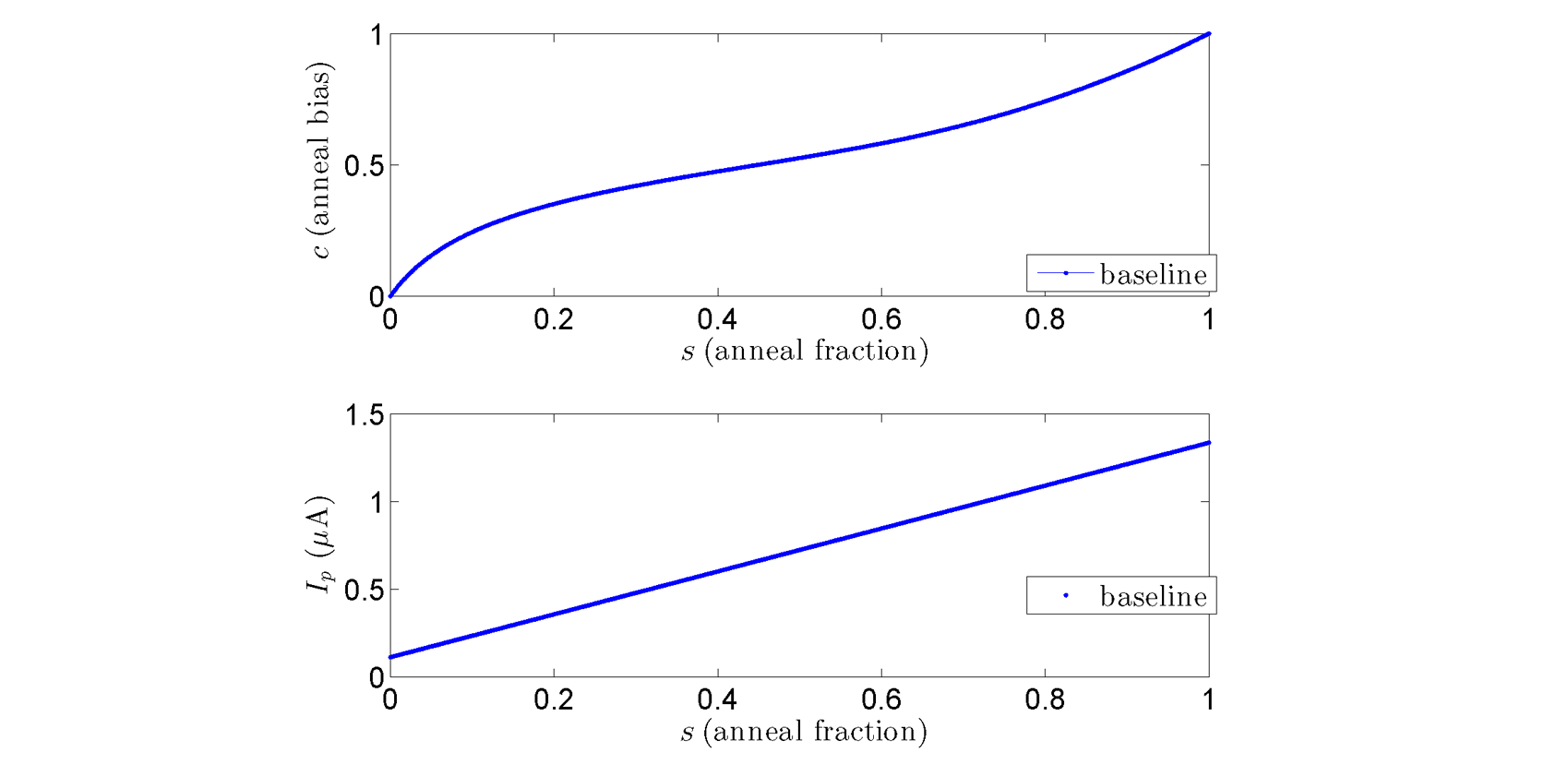
Fig. 87 Annealing control bias \(c\) versus anneal fraction \(s\). At \(c=0, s=0,\) \(A(s) \gg B(s)\), and at \(c=1, s=1, A(s) \ll B(s).\) Data shown are representative of D‑Wave 2000Q™ systems.#
On-QPU DACs allow adjustments of static annealing offsets \(\delta c_i\) per qubit, thereby advancing or delaying the annealing signal locally for each. Figure 88 shows an example of the annealing control bias with \(\delta c_i = 0.05\) and \(\delta c_i = -0.05\). Note that the anneal offset is a vertical shift up or down in annealing control bias, not a shift in \(s\).
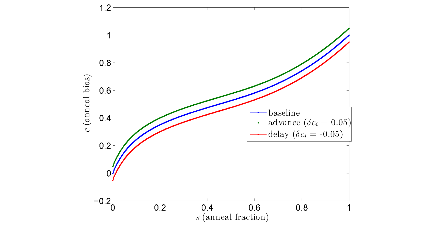
Fig. 88 Annealing control bias \(c\) versus anneal fraction \(s\) for several anneal offset values. Data shown are representative of D‑Wave 2000Q systems.#
Advancing or delaying the annealing bias by setting \(\delta c_i \ne 0\) changes the transverse field \(A_i(s)\) with respect to the original global \(A(s)\). This allows you to increase or decrease \(A_i(s)\). Note that \(\delta c_i > 0\) advances the annealing process (\(A_i(s) < A(s)\)) and \(\delta c_i < 0\) delays the annealing process (\(A_i(s) > A(s)\)). Figure 89 shows typical \(A_i(s)\) versus \(s\) for two values of \(\delta c_i\). Both \(A(s)\) and \(B(s)\) simultaneously change with control bias \(c\). Thus, a consequence of advancing or delaying the annealing process with anneal offset \(\delta c_i\) is that \(B(s)\rightarrow B_i(s)\). Figure 89 also shows typical \(B_i(s)\) versus \(s\) for the same set of \(\delta c_i\).
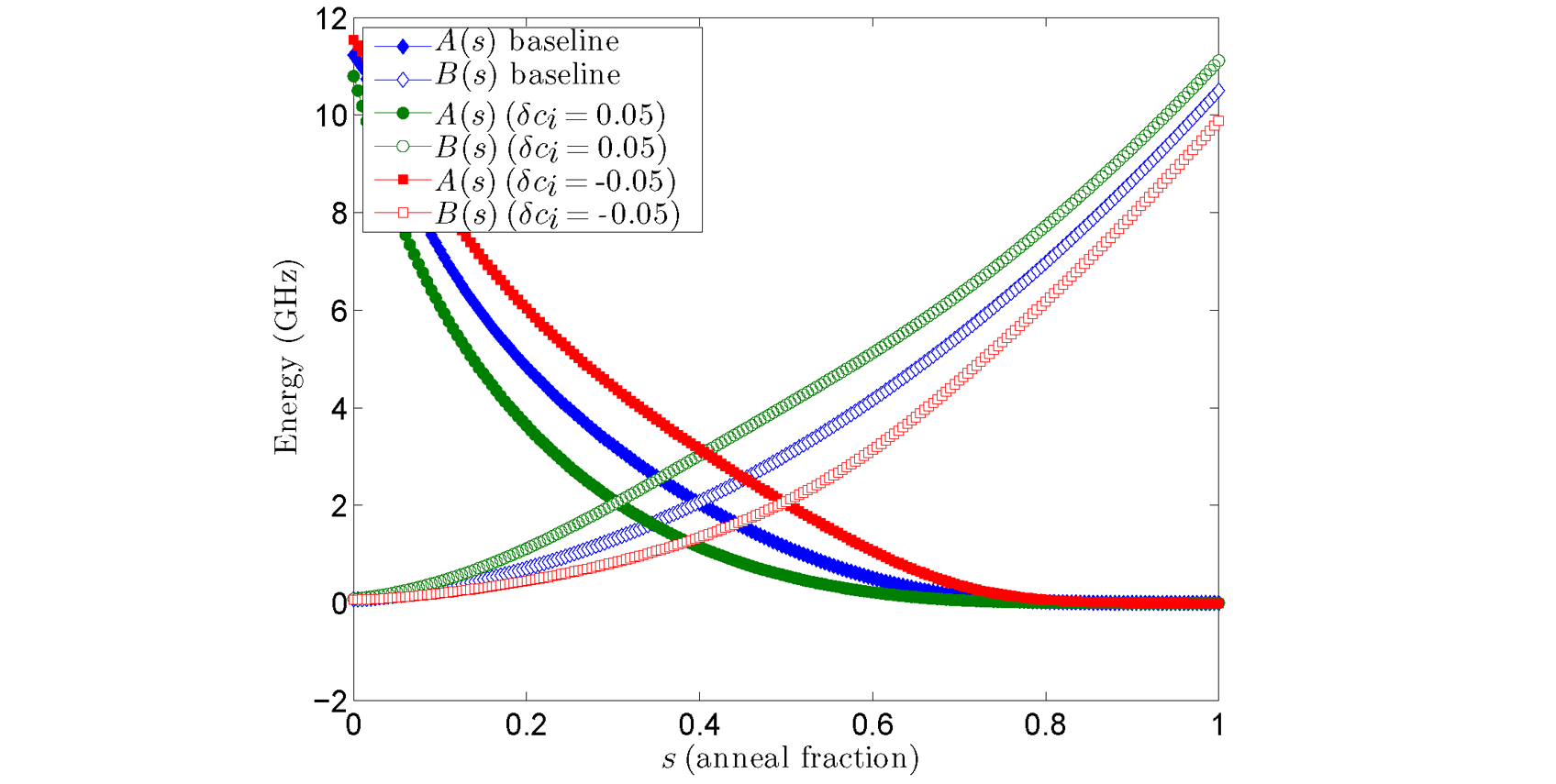
Fig. 89 \(A(s)\) and \(B(s)\) versus anneal fraction \(s\). At \(c(s=0)=0\), \(A(s) \gg B(s)\), and at \(c(s=1) = 1, A(s) \ll B(s)\). The baseline curve (\(\delta c_i = 0\)) is shown along with \(A_i(s), B_i(s)\) for anneal offset \(\delta c_i=0.05\) (advances the annealing process for the qubit) and \(A_i(s),B_i(s)\) for anneal offset \(\delta c_i = -0.05\) (delays the annealing process for the qubit). Data shown are representative of D‑Wave 2000Q systems.#
The change of \(B(s)\rightarrow B_i(s)\) has consequences for the target Ising spin Hamiltonian parameters \(h_i\) and \(J_{i,j}\). The anneal offset for the \(i{\rm th}\) qubit deflects \(h_i\rightarrow h_i(\delta c_i,s)\), and the anneal offsets for the \(i{\rm th}\) and \(j{\rm th}\) qubit deflect \(J_{i,j} \rightarrow J_{i,j}(\delta c_i,\delta c_j,s)\). Figure 90 shows plots of the bias \(h_i(\delta c_i,s)/h\) and coupling strength \(J_{i,j}(\delta c_i,0,s)/J\), both normalized by the values that would have been set without an applied offset, for several values of an offset \(\delta c_i\) applied to a single qubit. Figure 91 shows plots of \(J_{i,j}(\delta c_i,\delta c_j,s)/J\) for several values of offsets \(\delta c_i, \delta c_j\) applied to a pair of coupled qubits.
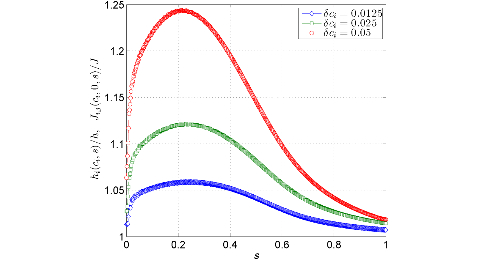
Fig. 90 \(h_i(\delta c_i, s)/h\) and \(J_{i,j}(\delta c_i,0, s)/J\) versus \(s\) for several values of \(\delta c_i\). The deviation of these quantities is \(s\)-dependent. You can choose a particular value of \(s\) at which to exactly compensate the change in target parameter by adjusting \(h_i(\delta c_i, s)\rightarrow h_i', J_{i,j}(\delta c_i,0, s) \rightarrow J_{i,j}'\). For values of \(s\) before or after this point, a residual change in target parameter remains. Data shown are representative of D‑Wave 2000Q systems.#
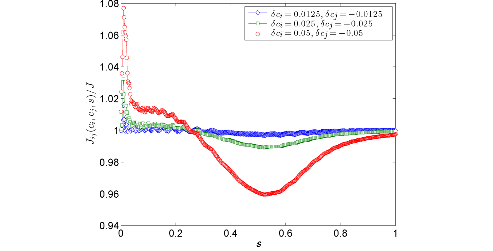
Fig. 91 \(J_{ij}(\delta c_i,\delta c_j, s)/J\) versus \(s\) for several values of \(\delta c_i\) and \(\delta c_j\). The deviation of these quantities away from 1 is \(s\)-dependent. You can choose a particular value of \(s\) at which to exactly compensate the change in target parameter by adjusting \(J_{i,j}(\delta c_i,\delta c_j, s)\rightarrow J_{i,j}'\). For values of \(s\) before or after this point, a residual change in target parameter remains. Data shown are representative of D‑Wave 2000Q systems.#
The changes shown in Figure 90 and Figure 91 are \(s\)-dependent. The largest changes are earlier in the annealing process. You can choose a particular value of \(s^*\) at which to exactly compensate these changes in target parameters by rescaling the requested target parameters. However, for values of \(s\) before or after \(s^*\), a residual change in target parameter remains.
Note
Where a two-state approximation holds well for the qubits (i.e., larger values of \(s\)), the effective Hamiltonian, rewritten following [Lan2017], can be approximated as:
where \(J_{i,j}\) and \(h_i\) are the programmed biases for the Ising model, and \(c(s)\) and \(c^{-1}\) are the smooth, monotonic normalized annealing bias and its inverse. You can determine all values of \(c(s)\) and \(c^{-1}\) by smoothly approximating (e.g. linear interpolation) the discretized form of \(c(s)\) available for QPUs on the QPU-Specific Characteristics page.
The impact of offsets can be interpreted as perturbations of \(J\) and \(h\) values relative to a fixed schedule,
For example, in the perturbative limit of small anneal offsets, a Taylor expansion yields:
Anneal offsets may improve results for problems in which the qubits have irregular dynamics for some easily determined reason. For example, if a qubit’s final value does not affect the energy of the classical state, you can advance it (with a positive offset) to reduce quantum bias in the system; see [Kin2016]. Anneal offsets can also be useful in embedded problems with varying chain length: longer chains may freeze out earlier than shorter ones—at an intermediate point in the anneal, some variables act as fixed constants while others remain undecided. If, however, you advance the anneal of the qubits in the shorter chains, they freeze out earlier than they otherwise would. The correct offset will synchronize the annealing trajectory of shorter chains with that of the longer ones. As a general rule, if a qubit is expected to be subject to a strong effective field relative to others, delay its anneal with a negative offset.
Determining the optimum offsets for different problem types is an area of research at D‑Wave. Expect that the appropriate offsets for two different qubits in the same problem to be within 0.2 normalized offset units of each other.
Varying the Global Anneal Schedule#
You can make changes to the global anneal schedule by submitting a set of points that define the piece-wise linear (PWL) waveform of the annealing pattern you want. You can change the standard (forward) schedule by introducing a pause or a quench, or you can initialize the qubits into a specific classical state and anneal in reverse from there. This section describes these features.
Pause and Quench#
Advantage systems provide user control over the global annealing trajectories:
You can scale the quadratic growth in persistent current—that is, quadratic growth in \(B(t)\)—using the annealing_time parameter.
You can also set the anneal_schedule parameter, which allows for a pause or quench partway through the annealing process.[4] A pause dwells for some time at a particular anneal fraction; a quench abruptly terminates the anneal within a few hundred nanoseconds of the point specified.
Unlike the anneal offsets feature—which allows you to control the annealing path of individual qubits separately—anneal schedule changes apply to all qubits in the working graph.
Changes to the schedule are controlled by a PWL waveform comprising \(n\) pairs of points. The first element is time \(t\) in microseconds; the second, the anneal fraction, \(s\), as a value between 0 and 1. This input causes the system to produce linear changes in \(s\) between \(s_i\) and \(s_{i+1}\).
The following rules apply to the set of anneal schedule points provided:
Time \(t\) must increase for all points in the schedule.
For forward annealing, the first point must be \((0, 0)\).
For reverse annealing, the anneal fraction \(s\) must start and end at \(s = 1\).
In the final point, anneal fraction \(s\) must equal 1 and time \(t\) must not exceed the maximum value in the annealing_time_range property.
The number of points must be \(\geq 2\).
The upper bound on the number of points is system-dependent; check the max_anneal_schedule_points property. For reverse annealing, the maximum number of points allowed is one more than the number given by this property.
The steepest slope of any curve segment, \(\frac{s_i - s_{i-1}}{t_i - t_{i-1}}\) must not be greater than the inverse of the minimum anneal time. For example, for a QPU with a annealing_time_range value of
[ 0.5, 2000 ], the minimum anneal time is 0.5 \(\mu s\), so the steepest supported slope is 2 \(\mu s^{-1}\). If you want a section of the piecewise-linear curve that starts at time point \(t_4 = 30 \mu s\) to increase from \(s_4=0.7\) to \(s_5=0.8\), this example QPU supports a schedule that contains \(t_5 = 30.06 \mu s\) ([... [30.0, 0.7], [30.06, 0.8], ...]), which has a maximum slope of \(1 \frac{2}{3}\), but not one that contains \(t_5 = 30.04 \mu s\) ([... [30.0, 0.7], [30.04, 0.8], ...]), which has a maximum slope of \(2 \frac{1}{2}\).Note that the I/O system that delivers the anneal waveform—the \(\Phi_{\rm CCJJ}(s)\) term of equation (3) in the QPU Solver Datasheet guide—to a QPU limits bandwidth with a 30 MHz low-pass filter for Advantage and Advantage2 systems; if you configure a too-rapidly changing curve, even with supported slopes, expect distorted values of h and J for your problem.
Only two points can be specified when fast_anneal is
True.
The table below gives three valid examples of anneal schedule points, producing the varying patterns of \(B(t)\) that appear in Figure 92.
Points |
Result |
|---|---|
\({(0.0, 0.0) (20.0, 1.0)}\) |
Standard trajectory of 20-\(\mu s\) anneal. Here, \(B(t)\) grows quadratically with time. |
\({(0.0, 0.0) (10.0, 0.5) (110.0, 0.5) (120.0, 1.0)}\) |
Mid-anneal pause at \(s = 0.5\). The quadratic growth of \(B(t)\) is interrupted by a 100-\(\mu s\) pause halfway through. |
\({(0.0, 0.0) (10.0, 0.5) (12.0, 1.0)}\) |
Mid-anneal quench at \(s = 0.5\). The quadratic growth of \(B(t)\) is interrupted by a rapid 2-\(\mu s\) quench halfway through. |

Fig. 92 Annealing schedule variations. Top: Standard quadratic growth of \(B\) for \(t_f = 20\ \mu s\). Middle: Mid-anneal pause of \(100\ \mu s\) at \(s = 0.5\) for a background \(t_f = 20\ \mu s\). Bottom: Mid-anneal quench of \(2\ \mu s\) at \(s = 0.5\) for a background \(t_f = 20\ \mu s\).#
This degree of control over the global annealing schedule allows you to study the quantum annealing algorithm in more detail. For example, a pause can be a useful diagnostic tool for instances with a small perturbative anticrossing. Figure 93 shows typical measurements of the 16-qubit instance reported in [Dic2013] with a pause inserted. While pauses early or late in the anneal have no effect, a pause near the expected perturbative anticrossing produces a large increase in the ground-state success rate.
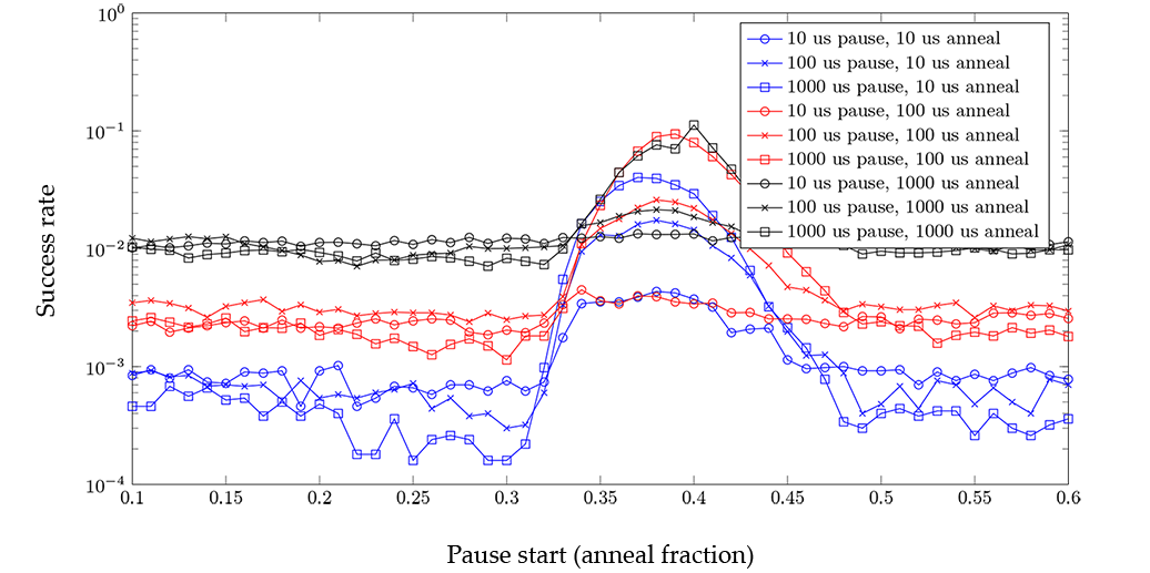
Fig. 93 Typical measurements from a 16-qubit reference instance showing pauses of different lengths inserted at different points in the annealing schedule. Pauses inserted near the expected anticrossing increase the likelihood of obtaining results from the ground state. Data shown are representative of D‑Wave 2000Q systems.#
Another example is a quench inserted at \(s < 1\). If the quench is fast compared to problem dynamics, then the distribution of states returned by the quench can differ significantly from that returned by the standard annealing schedule. Figure 94 shows typical measurements of the same 16-qubit instance with a quench added. The probability of obtaining ground state samples depends on when in the anneal the quench occurs, with later quenches more likely to obtain samples from the ground state.
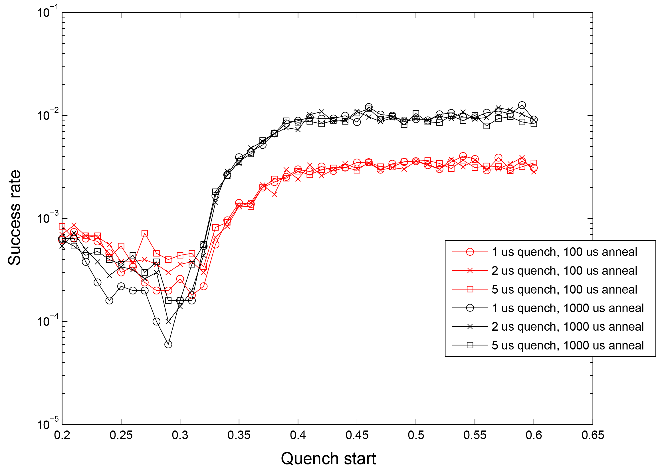
Fig. 94 Typical measurements from a 16-qubit reference instance showing quenches of different speeds compared to problem dynamics at different points in the anneal schedule. Later quenches increase the likelihood of obtaining results from the ground state. Data shown are representative of D‑Wave 2000Q systems.#
Reverse Annealing#
As described above, the annealing functions \(A(s)\) and \(B(s)\) are defined such that \(A(s) \gg B(s)\) at \(s=0\) and \(A(s) \ll B(s)\) at \(s = 1\), where \(s\) is the normalized annealing fraction. In the standard quantum annealing protocol, \(s\) increases linearly with time, with \(s(0)=0\) and \(s(t_f)=1\), where \(t_f\) is the total annealing time. The network of qubits starts in a global superposition over all possible classical states and, as \(s \rightarrow 1\), the system localizes into a single classical state; see Figure 81.
Reverse annealing allows you to initialize the qubits into a specific classical state, begin the evolution at \(s = 1\), anneal along a path toward \(s=0\), and then return back up to \(s=1\). Figure 95 shows a typical reverse annealing process where the system reverses to \(s = 0.5\), pauses for \(25 \ \mu s\) at \(s = 0.5\), and ends at \(s=1\).
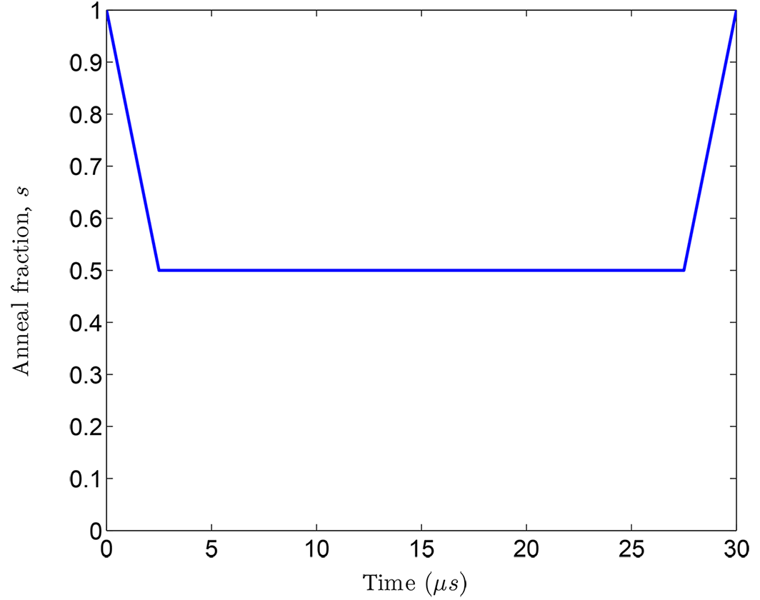
Fig. 95 Typical reverse annealing protocol with a \(5 \ \mu s\) equivalent ramp rate from \(s = 1\) to \(s = 0.5\), followed by a pause at \(s = 0.5\) for \(25 \ \mu s\), and then a ramp back to \(s = 1\).#
The reverse annealing feature gives you additional control over and insight into the quantum annealing process in the D‑Wave QPU.[5] Examples of how you might use reverse annealing include:
Quantum Boltzmann sampling—Prepare a classical state and then draw a set of samples from a probability distribution that may be changing with \(s\).
Hybrid algorithms—Prepare a classical state provided by a classical heuristic and then turn on a finite \(A(s)\) and allow the system to evolve.
Tunneling rate measurements—Prepare a particular classical state and measure the rate at which the system tunnels from this state to another for a range of \(s\).
Relaxation rate measurements—Prepare a classical state that is an excited state of the problem Hamiltonian and measure the rate at which the system relaxes to lower energy states for a range of \(s\).
The reverse annealing interface uses three parameters: anneal_schedule defines the waveform, \(s(t)\), and initial_state and reinitialize_state control the system state at the start of an anneal.
As for pause and quench, the reverse annealing schedule is controlled by a PWL waveform comprising \(n\) pairs of points. The first element of the pair is time \(t\) in microseconds; the second, the anneal fraction, \(s\), as a value between 0 and 1. Just as in forward annealing, time \(t\) must increase for all points in the schedule. For a reverse anneal, however, the anneal fraction must start and end at \(s = 1\).
The following table shows the tuples that you submit to get the pattern in Figure 95.
Points |
Result |
|---|---|
\({(0.0, 1) (2.5, 0.5) (27.5, 0.5) (30.0, 1.0)}\) |
Reverse anneal, therefore begins at \(s = 1\). A \(30.0 \ \mu s\) anneal with a mid-anneal pause at \(s = 0.5\) that lasts for \(25 \ \mu s\). |
When supplying a reverse annealing waveform through anneal_schedule, you must also supply the initial state to which the system is set. When multiple reads are requested in a single call to SAPI, you have two options for the starting state of the system. These are controlled by the reinitialize_state Boolean parameter:
reinitialize_state=true(default)—Reinitialize the initial state for every anneal-readout cycle. Each anneal begins from the state given in the initial_state parameter. Initialization time is required before every anneal-readout cycle. The amount of time required to reinitialize varies by system.reinitialize_state=false—Initialize only at the beginning, before the first anneal cycle. Each anneal (after the first) is initialized from the final state of the qubits after the preceding cycle. Initialization time is required only once.
The reinitialize_state parameter affects timing. See the Operation and Timing section for more information.
Fast Anneal#
Some QPUs support an alternate anneal protocol, the fast-anneal protocol, that enables you to execute an anneal within the coherent regime; for example, \(0 \le t \le t_f=7~\text{ns}\). This is the anneal protocol used in experiments such as [Kin2022].
Access this expanded range of annealing times by setting the fast_anneal
parameter to True. Provide the annealing timespan in either the
annealing_time or the anneal_schedule parameter. Anneal
times must be within the range specified by the fast_anneal_time_range property
for the selected QPU.
See the Fast-Anneal Protocol section for further details.