QPU Solvers: Decomposing Large Problems#
This chapter briefly presents methods of decomposing a large problem into a part requiring no more than the number of qubits available on the QPU and, optionally for hybrid approaches, parts suited to conventional compute platforms. Detailed information is available in the literature and referenced papers to guide actual implementation.
The dwave-hybrid package provides decomposition tools.
Energy-Impact Decomposing#
One approach to decomposition, implemented by the
EnergyImpactDecomposer class, is to select a
subproblem of variables maximally contributing to the problem energy.
The example illustrated in Figure 52 shows a large problem decomposed into smaller subproblems.
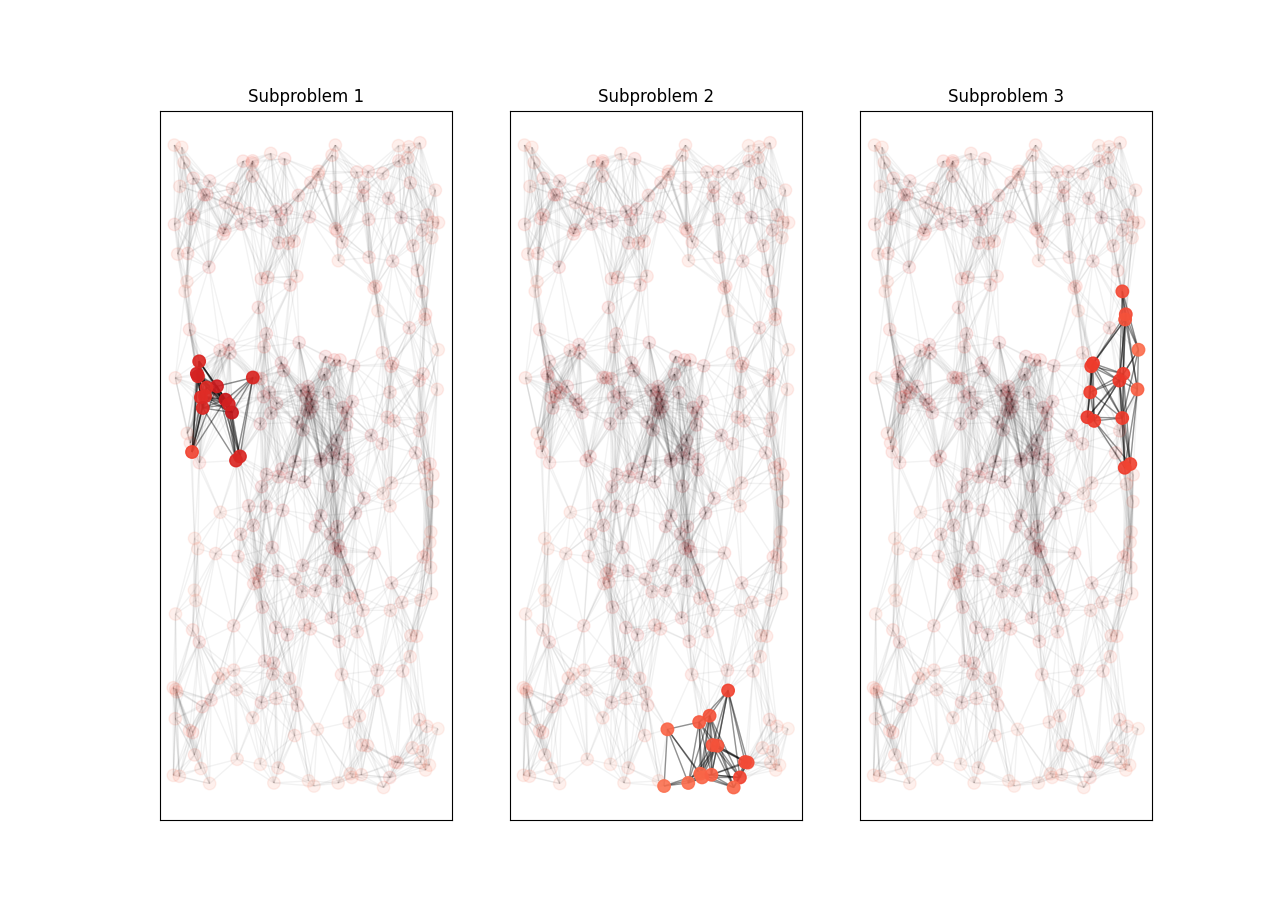
Fig. 52 A problem too large to be embedded in its entirety on the QPU is sequentially decomposed into smaller problems, each of which can fit on the QPU, with variables selected by highest impact on energy.#
Variables selected solely by maximal energy impact may not be directly connected (no shared edges) and might not represent a local structure of the problem. Configuring a mode of traversal such as breadth-first (BFS) or priority-first selection (PFS) can capture features that represent local structures within a problem.
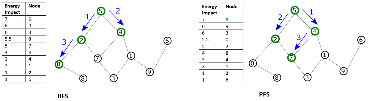
Fig. 53 BFS starts with the node with maximal energy impact, from which its graph traversal proceeds to directly connected nodes, then nodes directly connected to those, and so on, with graph traversal ordered by node index. In PFS, graph traversal selects the node with highest energy impact among unselected nodes directly connected to any already selected node.#
Example#
This example creates a hybrid decomposer that uses breadth-first traversal from the variable with the largest energy impact, selecting 50 variables for each subproblem.
>>> from hybrid.decomposers import EnergyImpactDecomposer
...
>>> decomposer = EnergyImpactDecomposer(size=50,
...                                     rolling_history=0.85,
...                                     traversal="bfs")
Further Information#
The dwave-hybrid package explains energy-impact decomposition and shows implementation examples.
Cutset Conditioning#
Cutset conditioning conditions on a subset of variables (the “cutset”) of a graph, leaving the remaining network as a tree with complexity that is exponential in the cardinality (size) of the cutset.
Chose a subset \(\setminus A\) of variables \(A\) to fix throughout the algorithm so that the graph of \(E(\vc{s}_A,\vc{s}_{\setminus A})\), where \(\argmin_{\vc{s}_A} E(\vc{s}_A,\vc{s}_{\setminus A})\) is the optimal setting of \(\vc{s}_A\) for a given \(\vc{s}_{\setminus A}\), breaks into separate components that can be solved independently:
where \(\vc{s}_A = \bigcup_\alpha \vc{s}_{A_\alpha}\) and \(\vc{s}_{A_\alpha} \cap \vc{s}_{A_{\alpha'}}=\emptyset\) for \(\alpha \not = \alpha'\).
Choose a cutset such that each of the remaining \(\min_{\vc{s}_{A_\alpha}}\) problems is small enough to be solved on the D‑Wave QPU.
Example#
A small example is illustrated in Figure 54.
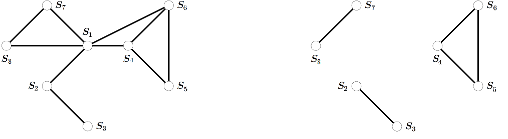
Fig. 54 8-variable graph, before (left) and after (right) conditioning. If the graph is conditioned on variable \(s_1\), it decomposes into 3 smaller subproblems. The remaining variable sets \(\vc{s}_A=\{s_2,s_3\}\cup\{s_4,s_5,s_6\}\cup \{s_7,s_8\}\) define three decoupled subproblems.#
To simplify outer optimization, make the number of conditioned variables as small as possible.
Further Information#
Branch-and-Bound Algorithms#
Branch-and-bound algorithms progressively condition more variables to either \(s_i=-1\) or \(s_i=1\), for spins, defining a split at node \(s_i\). Further splits define a branching binary tree with leaves defining the \(2^N\) configurations where all variables are assigned values. At each node a branch is pruned if no leaf node below it can contain the global optimum.
Example: Best Completion Estimate#
Branch-and-bound can benefit from using the D‑Wave system to terminate searches higher in the tree.
Condition sufficient variables so the remaining can be optimized by the QPU. Instead of exploring deeper, call the QPU to estimate the best completion from that node. As the upper bound is minimized through subsequent QPU completions, this may in turn allow for future pruning.
Note
Since the QPU solution does not come with a proof of optimality, this algorithm may not return a global minimum.
Example: Lower Bounds#
The D‑Wave system can also provide tight lower-bound functions at any node in the search tree.
Lagrangian relaxation finds these lower bounds by first dividing a node in the graph representing variable \(s_i\) in two (\(s_i^{(1)}\) and \(s_i^{(2)}\)) with constraint \(s_i^{(1)} = s_i^{(2)}\). The original objective \(E(s_i,\vc{s}_{\setminus i})\) becomes \(E'(s_i^{(1)}, s_i^{(2)},\vc{s}_{\setminus i})\), leaving the problem unchanged. With sufficient divided variables to decompose \(E'\) into smaller independent problems the equality constraints are softened and treated approximately:
The Lagrangian for the constrained problem is
Where \(\lambda_i\) is a multiplier for the equality constraint. Maximizing the dual function with respect to \(\lambda_i\),
provides the tightest possible lower bound.
Introduce enough divided variables to generate subproblems small enough to solve on the QPU and then optimize each subproblem’s dual function using a subgradient method to provide the tightest possible lower bounds.
As an example, consider again the small 8-variable problem, shown on the left side in Figure 55.
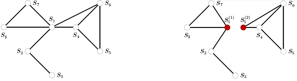
Fig. 55 8-variable graph, before (left) and after (right) splitting.#
The Lagrangian relaxed version of the problem obtained by dividing variable \(s_1\) is shown on the right. The constraint \(s_1^{(1)}=s_1^{(2)}\) is treated softly giving two independent subproblems consisting of variable sets \({s_1^{(1)}, s_2, s_3, s_7, s_8}\) and \({s_1^{(2)}, s_4, s_5, s_6}\). If either subproblem is still too large, it can be decomposed further either through another variable division or through conditioning.
Further Information#
[Bac2018] provides a method for verifying the output of quantum optimizers with ground-state energy lower bounds; notably, each step in the process requires only an effort polynomial in the system size.
[Bor2008] provides a max-flow approach to improved lower bounds for quadratic unconstrained binary optimization (QUBO).
[Boy2007] gives a concise introduction to subgradient methods.
[Bru1994] describes applying the branch-and-bound algorithm to the job shop scheduling problem.
[Glo2017] discusses preprocessing rules that reduce graph size.
[Ham1984] discusses roof duality, complementation and persistency in quadratic 0–1 optimization.
[Joh2007] gives an alternative to subgradient optimization, which examines a smooth approximation to dual function.
[Mar2007] considers ways to explore the search tree, including dynamic variable orderings and best-first orderings.
[Mon2020] describes a quantum algorithm that can accelerate classical branch-and-bound algorithms.
[Nar2017] propose a decomposition method more effective than branch-and-bound, which is implemented for the maximum clique problem.
[Ron2016] provides a method for solving constrained quadratic binary problems via quantum adiabatic evolution.
[Ros2016] discusses branch-and-bound heuristics in the context of the D‑Wave Chimera architecture.
Large-Neighborhood Local Search Algorithms#
Local search algorithms improve upon a candidate solution, \(\vc{s}^t\), available at iteration \(t\) by searching for better solutions within some local neighborhood of \(\vc{s}^t\).
Quantum annealing can be very simply combined with local search to allow the local search algorithm to explore much larger neighborhoods than the standard 1-bit-flip Hamming neighborhood.
For a problem of \(N\) variables and a neighborhood around configuration \(\vc{s}^t\) of all states within Hamming distance \(d\) of \(\vc{s}^t\), choose one of \(\binom{N}{d}\), and determine the best setting for these \(\vc{s}_A\) variables given the fixed context of the conditioned variables \(\vc{s}^{t}_{\setminus A}\). Select \(d\) small enough to solve on the QPU. If no improvement is found within the chosen subset, select another.
Further Information#
[Ahu2000] describes the cyclic exchange neighborhood, a generalization of the two-exchange neighborhood algorithm.
[Glo1990] is a tutorial on the tabu search algorithm.
[Liu2005] presents promising results for even small neighborhoods of size \(d\le 4\).
[Mar2018] proposes a variable neighbourhood search heuristic for the conformational problem, the three-dimensional spatial arrangements of constituent atoms of molecules.
Belief Propagation#
The belief propagation algorithm passes messages between regions and variables that represent beliefs about the minimal energy conditional on each possible value of a variable. It can be used, for example, to calculate approximate, and in some cases exact, marginal probabilities in Bayes nets.