Unconstrained Example: Solving a SAT Problem

The D-Wave quantum computer is well suited to solving optimization and satisfiability (SAT) problems with binary variables. Binary variables can only have values 0 (NO, or FALSE) or 1 (YES, or TRUE), which are easily mapped to qubit final states of “spin up” (\(\uparrow\)) and “spin down” (\(\downarrow\)). These are problems that answer questions such as, “Should a package be shipped on this truck?”

This section uses an example problem of a very simple SAT:

\[(x_1 \vee \overline{x}_2 ) \wedge (\overline{x}_1 \vee x_2)\]

This is a 2-SAT in conjunctive normal form (CNF), meaning it has disjunctions of two Boolean variables (\(X\) OR \(Y\)) joined by an AND, and is satisfied only if all its disjunctions are satisfied; that is, to make the SAT true, you must find and assign appropriate values of 0 or 1 to all its variables.

You can easily verify that the solution to this example problem is \(x_1=x_2\). For example:

\[\begin{split} x_1 = x_2=0 \quad \rightarrow \qquad (0 \vee 1) \wedge (1 \vee 0) = 1 \wedge 1 = 1 \\ x_1 {=} 0 \ \ne \ x2 {=} 1 \quad \rightarrow \qquad (0 \vee 0) \wedge (1 \vee 1) = 0 \wedge 1 = 0\end{split}\]

Note

The simple program below poses and solves this SAT in an alternative format familiar to anyone with some programming experience:

>>> import itertools
>>> def sat(x1, x2):
...     return (x1 or not x2) and (not x1 or x2)
>>> for (x1, x2) in list(itertools.product([False, True], repeat=2)):
...     print(x1, x2, '-->', sat(x1, x2))
False False --> True
False True --> False
True False --> False
True True --> True

Formulating an Objective Function

The first step in solving problems on QPU solvers is to formulate an objective function. Such an objective, usually in Ising or QUBO format, represents good solutions to the problem as low-energy states of the system. This subsection shows an intuitive approach to formulating such a QUBO.

For two variables, the QUBO formulation reduces to,

\[\text{E}(a_i, b_{i,j}; q_i) = a_1 q_1 + a_2 q_2 + b_{1,2} q_1 q_2,\]

where \(a_1\) and \(a_2\), the linear coefficients, and \(b_{1,2}\), the quadratic coefficient, are the programmable parameters you need to set so that \(q_1\) and \(q_2\), the binary variables (values of \(\{0,1\}\)), represent solutions to your problem when the objective function is minimized. For this simple example, it’s easy to work out values for these parameters.

A two-variable QUBO can have four possible values of its variables, representing four possible states of the system, as shown here:

State	\(q_1\)	\(q_2\)
1	0	0
2	0	1
3	1	0
4	1	1

For this objective function to represent the example SAT (i.e., to reformulate the original problem as an objective function that can be solved through minimization by a D-Wave solver), it needs to favor states 1 and 4 over states 2 and 3. You do this by penalizing states that do not satisfy the SAT; that is, by formulating the objective such that those states have higher energy.

First, notice that when \(q_1\) and \(q_2\) both equal 0—state 1—the value of the objective function is 0 for any value of the coefficients. To favor this state, you should formulate the objective function to have a global minimum energy (the ground state energy of the system) equal to 0. Doing so ensures that state 1 is a good solution.

Second, you penalize states 2 and 3 relative to state 1. One way to do this is to set both \(a_1\) and \(a_2\) to a positive value such as 0.1[1]. Doing so sets the the value of the objective function for those two states to \(0.1\).

[1]

Why not \(0.2\) or \(0.5\)? The Appendix: Next Learning Steps chapter looks at scaling the problem values.

Third, you also favor state 4 along with state 1. Given that for state 4, your objective function so far is

\[\text{E}(a_i=0.1, b_{i,j}; q_i=1) = 0.2 + b_{1,2},\]

you can do this by setting the quadratic coefficient \(b_{1,2} = -0.2\). The resulting objective function is

\[\text{E}(q_i) = 0.1 q_1 + 0.1 q_2 - 0.2 q_1 q_2,\]

and the table of possible outcomes is shown below.

State	\(q_1\)	\(q_2\)	Objective Value
1	0	0	0
2	0	1	0.1
3	1	0	0.1
4	1	1	0

Minor Embedding

You can represent this QUBO as the graph shown in Figure 29.

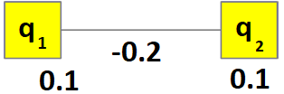
Fig. 29 Objective function for the example SAT problem.

This graph can be mapped to any two QPU qubits with a shared coupler. The Constraints Example: Problem Formulation chapter shows minor-embedding for less simple graphs.

Solving on a QPU

To program a D-Wave quantum computer is to set values for its qubit biases and coupler strengths. Configuring qubit biases of \(0.1\) for the two qubits found by minor embedding and a strength of \(-0.2\) for the shared coupler, and submitting to a QPU solver with a request for many anneals—also known as samples or reads—should strongly favor ground states 1 and 4 over excited states 2 and 3 in the returned results.

Below are results from running this problem on a Advantage system with the number of requested anneals set to 10,000:

Energy	State	Occurrences
0	1	4646
0	4	5349
0.1	2	2
0.1	3	3

If you run this problem again, you can expect the numbers associated with energy 0 to vary, but to stay near the number 5,000 (50% of the samples). In a perfect system, neither of the ground states should dominant over the other in a statistical sense; however, each run yields different numbers.

Notice that calling the QPU enough times occasionally returns excited states 2 and 3.

The next example shows how, exactly, you submit your problem to a D-Wave solver.