Workflow: Formulation and Sampling

This section provides a high-level description of how you solve problems using quantum computers.

The two main steps of solving problems using quantum computers are:

1. Formulate your problem as an objective function

   Objective (cost) functions are mathematical expressions of the problem to be optimized; for quantum computing, these are quadratic and nonlinear models that have lowest values (energy) for good solutions to the problems they represent.

2. Find good solutions by sampling

   Samplers are processes that sample from low-energy states of objective functions. Find good solutions by submitting your quadratic or nonlinear model to one of a variety of D‑Wave’s quantum, classical, and hybrid quantum-classical samplers.

Note

Samplers run—either remotely (for example, in D‑Wave’s Leap service) or locally on your CPU—on compute resources known as solvers. (Note that some classical samplers actually brute-force solve small problems rather than sample, and these are also referred to as solvers.)

Objective Functions

To express a problem for a D‑Wave solver in a form that enables solution by minimization, you need an objective function, a mathematical expression of the energy of a system. When the solver is a QPU, the energy is a function of binary variables representing its qubits; for quantum-classical hybrid solvers, the objective function might be more abstract.

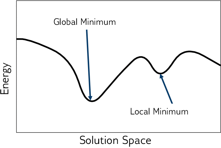
Fig. 4 Energy of the objective function.

For most problems, the lower the energy of the objective function, the better the solution. Sometimes any low-energy state is an acceptable solution to the original problem; for other problems, only optimal solutions are acceptable. The best solutions typically correspond to the global minimum energy in the solution space; see Figure 4.

Simple Objective Example

As an illustrative example, consider solving a simple equation, \(x+1=2\), not by the standard algebraic techniques but by formulating an objective that at its minimum value assigns a value to the variable, \(x\), that is also a good solution to the original equation.

Taking the square of the subtraction of one side from another, you can formulate the following objective function to minimize:

\[ \begin{align}\begin{aligned}\text{E}(x) &= [2-(x+1)]^2\\&= (1-x)^2\end{aligned}\end{align} \]

In this case minimization, \(\min_x{(1-x)^2}\), seeks the shortest distance between the sides of the original equation, which occurs at equality (with the square eliminating negative distance).

The Simple Sampling Example example below shows an equally simple solution by sampling.

Models

To express your problem as an objective function and submit to a D‑Wave sampler for solution, you typically use one of the quadratic models[1] or nonlinear model[2] provided by Ocean software:

• Binary Quadratic Models are unconstrained[3] and have binary variables.

  BQMs are typically used for applications that optimize over decisions that could either be true (or yes) or false (no); for example, should an antenna transmit, or did a network node experience failure?

• Constrained Quadratic Models can be constrained and have binary, integer and real variables.

  CQMs are typically used for applications that optimize problems that might include real, integer and/or binary variables and one or more constraints.

• Discrete Quadratic Models are unconstrained and have discrete variables.

  DQMs are typically used for applications that optimize over several distinct options; for example, which shift should employee X work, or should the state on a map be colored red, blue, green or yellow?

• Nonlinear Models can be constrained and have binary and integer variables.

  This model is especially suited for use with decision variables that represent a common logic, such as subsets of choices or permutations of ordering. For example, in a traveling salesperson problem, permutations of the variables representing cities can signify the order of the route being optimized, and in a knapsack problem, the variables representing items can be divided into subsets of packed and not packed.

[1]

Quadratic functions have one or two variables per term. A simple example of a quadratic function is,

\[D = Ax + By + Cxy\]

where \(A\), \(B\), and \(C\) are constants. Single variable terms—\(Ax\) and \(By\) here—are linear with the constant biasing the term’s variable. Two-variable terms—\(Cxy\) here—are quadratic with a relationship between the variables.

Ocean software also provides support for higher order models, which are typically reduced to quadratic for sampling.

[2]

The nonlinear model represents a general optimization problem with an objective function and/or constraints over variables of various types.

[3]

Constraints for such models are typically represented by adding penalty models to the objective, as shown in the Constraints Example: Problem Formulation section.

Samplers

Samplers are processes that sample from low-energy states of objective functions. Having formulated an objective function that represents your problem (typically as a quadratic or nonlinear model), you sample it for solutions.

D‑Wave provides quantum, classical, and quantum-classical hybrid samplers that run either remotely (for example, in D‑Wave’s Leap service) or locally on your CPU.

• QPU Solvers

  D‑Wave currently supports Advantage quantum computers.

  This guide focuses on QPU solvers and provides examples of using quantum computers to solve problems.

• Quantum-Classical Hybrid Solvers

  Quantum-classical hybrid is the use of both classical and quantum resources to solve problems, exploiting the complementary strengths that each provides. For an overview of, and motivation for, hybrid computing, see: Medium Article on Hybrid Computing.

  D‑Wave provides two types of hybrid solvers: Leap service’s hybrid solvers, which are cloud-based hybrid compute resources, and hybrid solvers developed in Ocean software’s dwave-hybrid tool.

• Classical Solvers

  You might use a classical solver while developing your code or on a small version of your problem to verify your code.

  For information on classical solvers, see the Ocean software documentation.

Simple Sampling Example

As an illustrative example, consider solving by sampling the objective, \(\text{E}(x) = (1-x)^2\) found in the Simple Objective Example example above to represent equation, \(x+1=2\).

This example creates a simple sampler that generates 10 random values of the variable \(x\) and selects the one that produces the lowest value of the objective:

>>> import random
...
>>> x = [random.uniform(-10, 10) for i in range(10)]
>>> e = list(map(lambda x: (1-x)**2, x))
>>> best_found = x[e.index(min(e))]

One particular execution found this best solution:

>>> print('x_i = ' + ' , '.join(f'{x_i:.2f}' for x_i in x))     
x_i = 7.87, 1.79, 9.61, 2.37, 0.68, -2.93, 3.96, 1.30, -3.85, -0.13
>>> print('e_i = ' + ', '.join(f'{e_i:.2f}' for e_i in e))      
e_i = 47.23, 0.63, 74.19, 1.89, 0.10, 15.44, 8.77, 0.09, 23.50, 1.28
>>> print("Best solution found is {:.2f}".format(best_found))   
Best solution found is 1.30

Figure 5 shows the value of the objective function for the random values of \(x\) chosen in the execution above. The minimum distance between the sides of the original equation, which occurs at equality, has the lowest value (energy) of \(\text{E}(x)\).

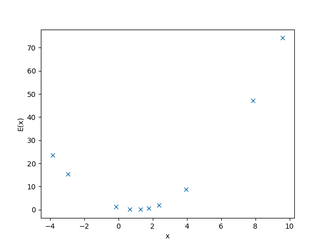
Fig. 5 Values of the objective function, \(\text{E}(x) = (1-x)^2\), versus random values of \(x\) selected by a simple random sampler.

Simple Workflow Example

This example uses Ocean software tools to demonstrate the solution workflow described in this section on a simple problem of finding the rectangle with the greatest area when the perimeter is limited.

In this example, the perimeter of the rectangle is set to 8 (meaning the largest area is for the \(2X2\) square).

A CQM is created that will have two integer variables, \(i, j\), each limited to half the maximum perimeter length of 8, to represent the lengths of the rectangle’s sides:

>>> from dimod import ConstrainedQuadraticModel, Integer
...
>>> i = Integer('i', upper_bound=4)
>>> j = Integer('j', upper_bound=4)
>>> cqm = ConstrainedQuadraticModel()

The area of the rectangle is given by the multiplication of side \(i\) by side \(j\). The goal is to maximize the area, \(i*j\). Because D‑Wave samplers minimize, the objective should have its lowest value when this goal is met. Objective \(-i*j\) has its minimum value when \(i*j\), the area, is greatest:

>>> cqm.set_objective(-i*j)

Finally, the requirement that the sum of both sides must not exceed the perimeter is represented as constraint \(2i + 2j <= 8\):

>>> cqm.add_constraint(2*i+2*j <= 8, "Max perimeter")
'Max perimeter'

Instantiate a hybrid CQM sampler and submit the problem for solution by a remote solver provided by the Leap quantum cloud service:

>>> from dwave.system import LeapHybridCQMSampler
...
>>> sampler = LeapHybridCQMSampler()                
>>> sampleset = sampler.sample_cqm(cqm)             
>>> print(sampleset.first)                          
Sample(sample={'i': 2.0, 'j': 2.0}, energy=-4.0, num_occurrences=1,
...            is_feasible=True, is_satisfied=array([ True]))

The best (lowest-energy) solution found has \(i=j=2\) as expected, a solution that is feasible because all the constraints (one in this example) are satisfied.

Quantum Samplers: What and How?

The Simple Workflow Example example above uses the Leap service’s hybrid CQM solver, which can accept integer variables and handle constraints natively. Hybrid samplers are also less restrictive on other aspects of the quadratic models they can accept; for example size (e.g., the number of variables) and structure (e.g., how interconnected the variables are).

This guide focuses on QPU solvers and provides examples of using quantum computers to solve problems:

• Chapter What is Quantum Annealing? explains the physics of how these quantum computers work as samplers.

• Chapter D‑Wave QPU Architecture: Topologies describes QPU topology, which can be helpful when mapping problem variables to qubits.

• Chapter Solving Problems with Quantum Samplers describes the particular workflow used for QPU solvers.

The guide’s other chapters walk you through simple examples of solving problems using this section’s workflow. Although a QPU solver is used, the introduction provided is useful for classical and hybrid solvers.