Operation and Timing

This section describes the computation process of D-Wave quantum computers, focusing on system timing, as follows:

• QMI Timing overviews the time allocated to a quantum machine instruction (QMI) while sections Service Time and QPU Access Time detail its parts, including the programming cycle and the anneal-read cycle of the D-Wave QPU.

• Usage Charge Time and Reported Time (Statistics) specify how solver usage is charged and reported in statistics for administrators.

• QMI Runtime Limit and Estimating Access Time explain the limits on QMI runtime duration and how to estimate the runtime for your problems.

• SAPI Timing Fields describes timing-related fields in the Solver API (SAPI).

• Timing Variation and Error describes sources of variation and error in timing.

QMI Timing

Fig. 105 shows a simplified diagram of the sequence of steps, the dark red set of arrows, to execute a quantum machine instruction (QMI) on a D-Wave system, starting and ending on a user’s client system. Each QMI consists of a single input together with parameters. A QMI is sent across a network to the SAPI server and joins a queue. Each queued QMI is assigned to one of possibly multiple workers, which may run in parallel. A worker prepares the QMI for the quantum processing unit (QPU) and postprocessing[1], sends the QMI to the QPU queue, receives samples (results) and post-processes them (overlapping in time with QPU execution), and bundles the samples with additional QMI-execution information for return to the client system.

[1]

Server-side postprocessing for Advantage systems is limited to computing the energies of returned samples. Ocean software provides additional client-side postprocessing tools.

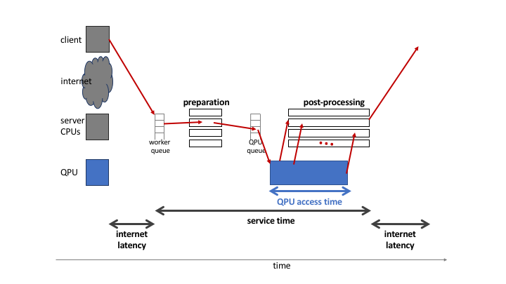
Fig. 105 Overview of execution of a single QMI, starting from a client system, and distinguishing classical (client, CPU) and quantum (QPU) execution.

The total time for a QMI to pass through the D-Wave system is the service time. The execution time for a QMI as observed by a client includes service time and internet latency. The QPU executes one QMI at a time, during which the QPU is unavailable to any other QMI. This execution time is known as the QMI’s QPU access time.

Service Time

The service time can be broken into:

• Any time required by the worker before and after QPU access

• Wait time in queues before and after QPU access

• QPU access time

• Postprocessing time

Service time is defined as the difference between the times of the QMI’s ingress (arrival at SAPI) and sample set’s egress (exit from the quantum computer) for each QMI.

Service time for a single QMI depends on the system load; that is, how many other QMIs are present at a given time. During periods of heavy load, wait time in the two queues may contribute to increased service times. D-Wave has no control over system load under normal operating conditions. Therefore, it is not possible to guarantee that service time targets can be met. Service time measurements described in other D-Wave documents are intended only to give a rough idea of the range of experience that might be found under varying conditions.

Viewing the Service Time for Your Problems

You can know the service time for a submitted problem by calculating the difference between its recorded egress and ingress times.

On the Leap dashboard, you can select a submitted problem (by your assigned label or its SAPI-assigned identifier) and view those times as shown here:

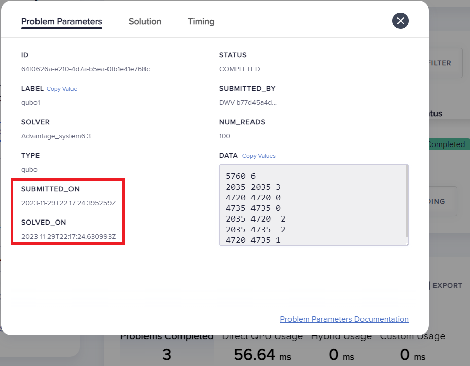
Fig. 106 Ingress and egress times for a problem in Leap.

Alternatively, you can retrieve this same information from SAPI in various ways, as demonstrated in the SAPI Timing Fields section and in examples in the SAPI REST Developer Guide.

Postprocessing Time

Server-side postprocessing for Advantage systems is limited to computing the energies of returned samples.[2] As shown in the Appendix: Benefits of Postprocessing section, more complex postprocessing can provide performance benefits at low timing cost. Ocean software provides such additional client-side postprocessing tools.

[2]

Earlier D-Wave systems, such as the D-Wave 2000Q system, optionally provided additional server-side postprocessing.

Figure 107 shows how a problem’s set of samples are batched and sent through the postprocessing solver as the next batch is being computed by the QPU. Server-side postprocessing works in parallel with sampling, so that the computation times overlap except for postprocessing the last batch of samples.

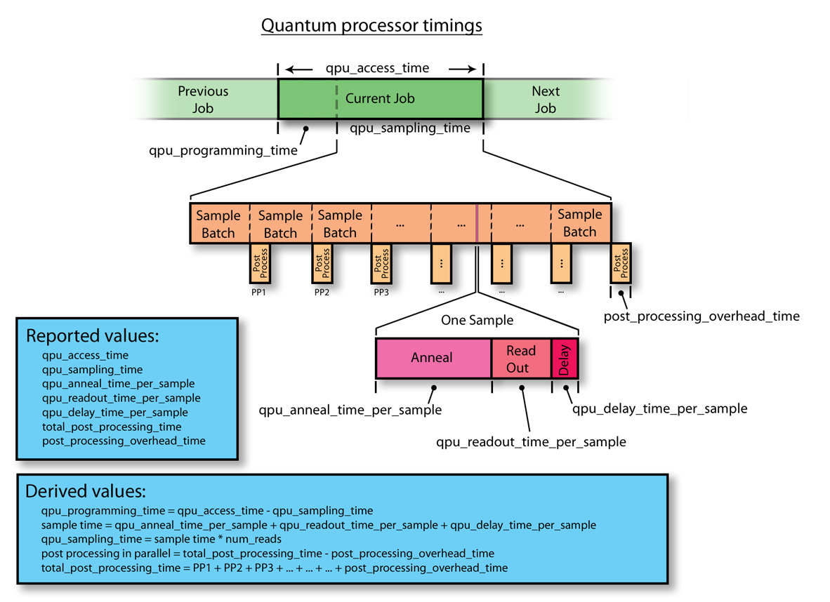
Fig. 107 Relationship of QPU time to postprocessing time, illustrated by one QMI in a sequence (previous, current, next).

Postprocessing overhead is designed not to impose any delay to QPU access for the next QMI, because postprocessing of the last batch of samples takes place concurrently with the next QMI’s programming time.

Viewing the Postprocessing Time for Your Problems

As shown in Fig. 107, total_post_processing_time is the sum of all times for the “Post Process” boxes while post_processing_overhead_time is the extra time needed (a single “Post Process” box) to process the last batch of samples. This latter time together with qpu_access_time contributes to overall service time.

On the Leap dashboard, you can click on a submitted problem identified by your assigned label or its SAPI-assigned identifier and see its postprocessing times. Alternatively, you can retrieve this same information from SAPI as demonstrated in the SAPI Timing Fields section.

QPU Access Time

As illustrated in Figure 108, the time to execute a single QMI on a QPU, QPU access time, is broken into two parts: a one-time initialization step to program the QPU (blue) and typically multiple sampling times for the actual execution on the QPU (repeated multicolor).

Fig. 108 Detail of QPU access time.

The QPU access time also includes some overhead:

\[T = T_p + \Delta + T_s,\]

where \(T_P\) is the programming time, \(T_s\) is the sampling time, and \(\Delta\) (reported as qpu_access_overhead_time by SAPI and not included in the qpu_access_time SAPI field that reports the QPU-usage time being charged) is an initialization time spent in low-level operations, roughly 10-20 ms for Advantage systems.

The time for a single sample is further broken into anneal (the anneal proper; green), readout (read the sample from the QPU; red), and thermalization (wait for the QPU to regain its initial temperature; pink). Possible rounding errors mean that the sum of these times may not match the total sampling time reported.

\[T_s / R \approx T_a + T_r + T_d,\]

where \(R\) is the number of reads, \(T_a\) the single-sample annealing time, \(T_r\) the single-sample readout time, and \(T_d\) the single-sample delay time, which consists of the following optional components[3]:

\[\begin{split}T_d = &readout\_thermalization \\ &+ reduce\_intersample\_correlation \\ &+ reinitialize\_state.\end{split}\]

[3]

See descriptions of these components under Solver Parameters. The reinitialize_state parameter is used only for reverse annealing.

Programming Cycle

When an Ising problem is provided as a set of h and J values,[4] the D-Wave system conveys those values to the DACs located on the QPU. Room-temperature electronics generate the raw signals that are sent via wires into the refrigerator to program the DACs. The DACs then apply static magnetic-control signals locally to the qubits and couplers. This is the programming cycle of the QPU.[5] After the programming cycle, the QPU is allowed to cool for a postprogramming thermalization time of, typically, 1 ms; see the Temperature section for more details about this cooling time.

[4]

Several other instructions to the system are provided by the user: for example, an annealing_time over which the quantum annealing process is to occur. See Solver Properties and Parameters Reference for details.

[5]

In some descriptions, the programming cycle is subdivided into a reset step that erases previous data stored in the DACs, followed by a programming step.

The total time spent programming the QPU, including the postprogramming thermalization time, is reported back as qpu_programming_time.

Anneal-Read Cycle

After the programming cycle, the system switches to the annealing phase during which the QPU is repeatedly annealed and read out. Annealing is performed using the analog lines over a time specified by the user as annealing_time and reported by the QPU as qpu_anneal_time_per_sample. Afterward, the digital readout system of the QPU reads and returns the spin states of the qubits. The system is then allowed to cool for a time returned by the QPU as qpu_delay_time_per_sample—an interval comprising a constant value plus any additional time optionally specified by the user via the readout_thermalization parameter.

The anneal-read cycle is also referred to as a sample. The cycle repeats for some number of samples specified by the user in the num_reads parameter, and returns one solution per sample. The total time to complete the requested number of samples is returned by the QPU as qpu_sampling_time.

Usage Charge Time

D-Wave charges you for time that solvers run your problems, with rates depending on QPU usage. You can see the rate at which your account’s quota is consumed for a particular solver in the solver’s quota_conversion_rate property.

You can see the time you are charged for in the responses returned for your submitted problems. The relevant field in the response is 'qpu_access_time'. The example in the SAPI Timing Fields section shows 'qpu_access_time': 9687 in the returned response, meaning almost 10 milliseconds are being charged.

For example, for a QPU solver with a quota conversion rate of 1, a problem that results in a 'qpu_access_time': 1500, deducts 1.5 milliseconds seconds from your account’s quota.

Reported Time (Statistics)

One timing parameter, qpu_access_time, provides the raw data for the “Total Time” values reported as system statistics, available to administrators. Reported statistics are the sum of the qpu_access_time values for each QMI selected by the users, solvers, and time periods selected in the filter.

Note

Reported statistics are in milliseconds, while SAPI inputs and outputs are in microseconds. One millisecond is 1000 microseconds.

QMI Runtime Limit

The D-Wave system limits your ability to submit a long-running QMI to prevent you from inadvertently monopolizing QPU time. This limit varies by system; check the problem_run_duration_range property for your solver.

The limit is calculated according to the following formula:

\begin{equation} Duration = ((P_1 + P_2) * P_3) + P_4 \end{equation}

where \(P_1\), \(P_2\), \(P_3\), and \(P_4\) are the values specified for the annealing_time, readout_thermalization, num_reads (samples), and programming_thermalization parameters, respectively.

If you attempt to submit a QMI whose execution time would exceed the limit for your system, an error is returned showing the values in microseconds. For example:

ERROR: Upper limit on user-specified timing related parameters exceeded: 12010000 > 3000000

Note that it is possible to specify values that fall within the permitted ranges for each individual parameter, yet together cause the time to execute the QMI to surpass the limit.

Keeping Within the Runtime Limit

If you are submitting long-duration problems directly to QPUs, you may need to make multiple problem submissions to avoid exceeding the runtime limit.[6] You can always divide the required number of reads among these submissions such that the runtime for each submission is equal to or less than the QPU’s runtime limit. For example, if a QPU has a runtime limit of 1,000,000 microseconds (1 second) and a problem has an estimated runtime of 3,750,000 microseconds for 1000 reads, the problem could be divided into four submissions of 250 reads each. (With spin-reversal transforms (SRTs), you similarly divide your samples into such batches; consider using Ocean software’s SpinReversalTransformComposite composite to also benefit from potential reduction in QPU biases.)

For a detailed breakdown of the QPU access-time estimates for your problem submission, see the Estimating Access Time section.

[6]

You could also adjust timing-related solver parameters. For information about solver parameters, see the Solver Parameters section.

Estimating Access Time

You can estimate a problem’s QPU access time from the parameter values you specify, timing data provided in the problem_timing_data solver property, and the number of qubits used to embed[7] the problem on the selected QPU.

Ocean software’s estimate_qpu_access_time() method implements the procedure described in the table below. The following example uses this Ocean method to estimate the QPU access time for a random problem with a 20-node complete graph using an anneal schedule that sets a ~1 ms pause on a D-Wave quantum computer. For the particular execution shown in this example, quantum computer system Advantage_system4.1 was selected, the required QPU access time for 50 samples found acceptable, and the problem then submitted to that quantum computer with the same embedding used in the time estimation.

>>> from dwave.system import DWaveSampler, FixedEmbeddingComposite
>>> from minorminer.busclique import find_clique_embedding
>>> import dimod
...
>>> # Create a random problem with a complete graph
>>> bqm = dimod.generators.uniform(20, "BINARY")
...
>>> # Select a QPU, find an embedding for the problem and the number of required qubits
>>> qpu = DWaveSampler()
>>> embedding = find_clique_embedding(bqm.variables, qpu.to_networkx_graph())  
>>> num_qubits = sum(len(chain) for chain in embedding.values())
...
>>> # Define the submission parameters and estimate the required time
>>> MAX_TIME = 500000   # limit single-problem submissions to 0.5 seconds
>>> num_reads = 50
>>> anneal_schedule = [[0.0, 0.0], [40.0, 0.4], [1040.0, 0.4], [1042, 1.0]]
>>> estimated_runtime = qpu.solver.estimate_qpu_access_time(num_qubits,
...    num_reads=num_reads, anneal_schedule=anneal_schedule)    
>>> print("Estimate of {:.0f}us on {}".format(estimated_runtime, qpu.solver.name))  
Estimate of 75005us on Advantage_system4.1
...
>>> # Submit to the same solver with the same embedding
>>> if estimated_runtime < MAX_TIME:
...    sampleset = FixedEmbeddingComposite(qpu, embedding).sample(bqm,
...       num_reads=num_reads, anneal_schedule=anneal_schedule)   

The following table provides a procedure for collecting the required information and calculating the runtime estimation for versions 1.0.x[8] of the timing model.

Table 35 Estimating the QPU Access Time for Problems

Row	QMI Time Component	Instruction
1	Typical programming time	Take the value from the typical_programming_time field.
2	Reverse annealing programming time	If reverse annealing is used, take the value from one of the the fields of the problem_timing_data solver property as follows: If the reinitialize_state parameter is specified as true, then take the value from reverse_annealing_with_reinit_prog_time_delta. If the reinitialize_state parameter is specified as false, then take the value from reverse_annealing_without_reinit_prog_time_delta. Otherwise, the value is 0.
3	Programming thermalization time	Take the value from either the the programming_thermalization solver parameter, if specified, or the default_programming_thermalization field.
4	Total programming time	Add rows 1–3.
5	Anneal time	Take the anneal time specified in the anneal_schedule or annealing_time solver parameter; otherwise, take the value from the default_annealing_time field.
6	Readout time	Calculate this value using the numpy functions numpy.interp() and numpy.emath.log10() and the Python function pow() as follows: If readout_time_model is pwl_log_log, then the following Python code can be used: pow(10, interp(log10(m), q, t)) If readout_time_model is pwl_linear, then the following Python code can be used: interp(m, q, t) where m is the number of qubits in the embedded problem and q = readout_time_model_parameters[0:N] and t = readout_time_model_parameters[N:2N] are the first N and last N elements of the 2N = len(readout_time_model_parameters) elements of the problem_timing_data solver property’s readout_time_model_parameters field.
7	Delay time	Take the value from the qpu_delay_time_per_sample field.
8	Reverse annealing delay time	If reverse annealing is used, take the value from one of the following fields of the problem_timing_data solver property: If the reinitialize_state parameter is specified as true, then take the value from reverse_annealing_with_reinit_delay_time_delta. If the reinitialize_state parameter is specified as false, then take the value from reverse_annealing_without_reinit_delay_time_delta.
9	Readout thermalization time	Take the value from either the readout_thermalization solver parameter, if specified, or the default_readout_thermalization solver property.
10	Decorrelation time	If the reduce_intersample_correlation solver parameter is specified as true, then the following Python code can be used to calculate the decorrelation time: a / m * (r[1] - r[0]) + r[0] where a is the anneal time (row 5), m is the decorrelation_max_nominal_anneal_time field, r[0] and r[1] are the first and last elements of the decorrelation_time_range field. If the reduce_intersample_correlation solver parameter is false, the value is 0.
11	Sampling time per read	Add rows 5–8 and the larger of either row 9 or 10.
12	Number of reads	Take the value from the num_reads solver parameter.
13	Total sampling time	Multiply row 11 by row 12.
14	QPU access time	Add row 4 and 13.

[7]

Embedding is typically heuristic and the number of required qubits can vary between executions. If you are using a heuristic embedding tool such as minorminor indirectly through your sampler (e.g., by using Ocean’s EmbeddingComposite or DWaveCliqueSampler), you can use the same tool on your problem to estimate the expected number of qubits: for large, complex problems you might run the tool several times and take the number of qubits from the produced average or worst-case embedding; for small, simple problems even a single run might be sufficient. If you are using such a tool directly (e.g., in conjunction with Ocean’s FixedEmbeddingComposite) or otherwise generating a heuristic or non-heuristic embedding, take the required number of qubits from your embedding. Because embedding depends on a QPU’s working graph, such embeddings should be for the particular QPU for which you are estimating the access time.

[8]

The version is specified in the problem_timing_data solver property.

SAPI Timing Fields

The table below lists the timing-related fields available in D-Wave’s Ocean SDK. Ocean users access to this information is from the info field in the dimod sampleset class, as in the example below. Note that the time is given in microseconds with a resolution of at least 0.01 \(\mu s\).[9]

[9]

Time resolution is higher for some fields, such as qpu_anneal_time_per_sample, which can be meaningful when the fast-anneal protocol is used.

>>> from dwave.system import DWaveSampler, EmbeddingComposite
>>> sampler = EmbeddingComposite(DWaveSampler())
>>> sampleset = sampler.sample_ising({'a': 1}, {('a', 'b'): 1})
>>> print(sampleset.info["timing"])   
{'qpu_sampling_time': 80.78,
 'qpu_anneal_time_per_sample': 20.0,
 'qpu_readout_time_per_sample': 39.76,
 'qpu_access_time': 16016.18,
 'qpu_access_overhead_time': 10426.82,
 'qpu_programming_time': 15935.4,
 'qpu_delay_time_per_sample': 21.02,
 'total_post_processing_time': 809.0,
 'post_processing_overhead_time': 809.0}

Table 36 Fields that affect qpu_access_time

QMI Time Component	SAPI Field Name	Meaning	Affected by
\(T\)	qpu_access_time	Total time in QPU	All parameters listed below
\(T_p\)	qpu_programming_time	Total time to program the QPU[10]	programming_thermalization, weakly affected by other problem settings (such as \(h\), \(J\), anneal_offsets, flux_offsets, and h_gain_schedule)
\(\Delta\)		Time for additional low-level operations
\(R\)		Number of reads (samples)	num_reads
\(T_s\)	qpu_sampling_time	Total time for \(R\) samples	num_reads, \(T_a\), \(T_r\), \(T_d\)
\(T_a\)	qpu_anneal_time_per_sample	Time for one anneal	anneal_schedule, annealing_time
\(T_r\)	qpu_readout_time_per_sample	Time for one read	Number of qubits read[11]
\(T_d\)	qpu_delay_time_per_sample	Delay between anneals[12]	anneal_schedule, readout_thermalization, reduce_intersample_correlation, (only in case of reverse annealing), reinitialize_state
	total_post_processing_time	Total time for postprocessing	Programming time
	post_processing_overhead_time	Extra time needed to process the last batch	total_post_processing_time

[10]

Even if programming_thermalization is 0, \(T_p\) is typically between 10 and 20 ms depending on processor and describes the time spent setting the \(h\) and \(J\) parameters of the problem as well as other features such as anneal_offsets, flux_offsets, h_gain_schedule.

[11]

The time to read a sample set from a Advantage generation QPU depends on the location of the qubits on the processor and the number of qubits in the sample set: a problem represented by a dozen qubits has shorter read times (and so a shorter \(T_r\), the total_readout_time) than a problem represented by several thousand qubits.

For the Advantage QPU, this can be significant. For example, some small problems may take \(25\ \mu s\) per read while a large problem might take \(150\ \mu s\) per read.

[12]

The time returned in the qpu_delay_time_per_sample field is equal to a constant plus the user-specified value, readout_thermalization.

Timing Data Returned by dwave-cloud-client

Below is a sample skeleton of Python code for accessing timing data returned by dwave-cloud-client. Timing values are returned in the computation object and the timing object; further code could query those objects in more detail. The timing object referenced on line 16 is a Python dictionary containing (key, value) pairs. The keys match keywords discussed in this section.

01 import random
02 import datetime as dt
03 from dwave.cloud import Client

04 # Connect using the default or environment connection information
05 with Client.from_config() as client:

06     # Load the default solver
07     solver = client.get_solver()

08     # Build a random Ising model to exactly fit the graph the solver supports
09     linear = {index: random.choice([-1, 1]) for index in solver.nodes}
10     quad = {key: random.choice([-1, 1]) for key in solver.undirected_edges}

11     # Send the problem for sampling, include solver-specific parameter 'num_reads'
12     computation = solver.sample_ising(linear, quad, num_reads=100)
13     computation.wait()

14     # Print the first sample out of a hundred
15     print(computation.samples[0])
16     timing = computation['timing']


17     # Service time
18     time_format = "%Y-%m-%d %H:%M:%S.%f"
19     start_time = dt.datetime.strptime(str(computation.time_received)[:-6], time_format)
20     finish_time = dt.datetime.strptime(str(computation.time_solved)[:-6], time_format)
21     service_time = finish_time - start_time
22     qpu_access_time = timing['qpu_access_time']
23     print("start_time="+str(start_time)+", finish_time="+str(finish_time)+ \
24             ", service_time="+str(service_time)+", qpu_access_time="       \
25             +str(float(qpu_access_time)/1000000))

Timing Variation and Error

Running a D-Wave-using program across the internet or even examining QPU timing information may show variation from run to run from the end-user’s point of view. This section describes some of the possible sources of such variation.

Nondedicated QPU Use

D-Wave systems are typically shared among multiple users, each of whom submits QMIs to solve a problem, with little to no synchronization among users. (A single user may also have multiple client programs submitting unsynchronized QMIs to a D-Wave system.) The QPU must be used by a single QMI at a time, so the D-Wave system software ensures that multiple QMIs flow through the system and use the QPU sequentially. In general, this means that a QMI may get queued for the QPU or some other resource, injecting indeterminacy into the timing of execution.

Note

Contact your D-Wave system administrator or D-Wave Customer Support if you need to ensure a quiet system.

Nondeterminacy of Classical System Timings

Even when a system is quiet except for the program to be measured, timings often vary. As illustrated in Fig. 109, running a given code block repeatedly can yield different runtimes on a classical system, even though the instruction execution sequence does not change. Runtime distributions with occasional large outliers, as seen here, are not unusual.

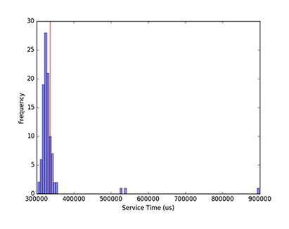
Fig. 109 Histogram of 100 measurements of classical execution time using a wall clock timer, showing that the mean time of 336.5 ms (red line) is higher than 75 percent of the measurements.

Timing variations are routine, caused by noise from the operating system (e.g., scheduling, memory management, and power management) and the runtime environment (e.g., garbage collection, just-in-time compilation, and thread migration). [13] In addition, the internal architecture of the classical portion of the D-Wave system includes multiple hardware nodes and software servers, introducing communication among these servers as another source of variation.

For these reasons, mean reported runtimes can often be higher than median runtimes: for example, in Fig. 109, the mean time of 336.5 ms (vertical red line) is higher than 75 percent of the measured runtimes due to a few extreme outliers (one about 3 times higher and two almost 2 times higher than median). As a result, mean runtimes tend to exceed median runtimes. In this context, the smallest time recorded for a single process is considered the most accurate, because noise from outside sources can only increase elapsed time.[14] Because system activity increases with the number of active QMIs, the most accurate times for a single process are obtained by measuring on an otherwise quiet system.

Note

The 336 ms mean time shown for this particular QMI is not intended to be representative of QMI execution times.

The cost of reading a system timer may impose additional measurement errors, since querying the system clock can take microseconds. To reduce the impact of timing code itself, a given code block may be measured outside a loop that executes it many times, with running time calculated as the average time per iteration. Because of system and runtime noise and timer latency, component times measured one way may not add up to total times measured another way.[15] These sources of timer variation or error are present on all computer systems, including the classical portion of D-Wave platforms. Normal timer variation as described here may occasionally yield atypical and imprecise results; also, one expects wall clock times to vary with the particular system configuration and with system load.

[13]

A more common practice in computational research is to report an alternative measurement called CPU time, which is intended to filter out operating system noise. However, CPU timers are only accurate to tens of milliseconds, and CPU times are not available for QPU time measurements. For consistency, we use wall clock times throughout.

[14]

Randal E. Bryant and David R. O’Hallaron, Computer Systems: A Programmer’s Perspective (2nd Edition), Pearson, 2010.

[15]

Paulo Eduardo Nogueira, Rivalino Matias, Jr., and Elder Vicente, An Experimental Study on Execution Time Variation in Computer Experiments, ACM Symposium on Applied Computing, 2014.

Internet Latency

If you are running your program on a client system geographically remote from the D-Wave system on which you’re executing, you will likely encounter latency and variability from the internet connection itself (see Fig. 105).

Settings of User-Specified Parameters

The following user-specified parameters can cause timing to change, but should not affect the variability of timing. For more information on these parameters, see Solver Properties and Parameters Reference.

• anneal_schedule—User-provided anneal schedule. Specifies the points at which to change the default schedule. Each point is a pair of values representing time \(t\) in microseconds and normalized anneal fraction \(s\). The system connects the points with piecewise-linear ramps to construct the new schedule. If anneal_schedule is specified, \(T_a\), qpu_anneal_time_per_sample is populated with the total time specified by the piecewise-linear schedule.

• annealing_time—Duration, in microseconds, of quantum annealing time. This value populates \(T_a\), qpu_anneal_time_per_sample.

• num_reads—Number of samples to read from the solver per QMI.

• programming_thermalization—Number of microseconds to wait after programming the QPU to allow it to cool; i.e., post-programming thermalization time. Values lower than the default accelerate solving at the expense of solution quality. This value contributes to the total \(T_p\), qpu_programming_time.

• readout_thermalization—Number of microseconds to wait after each sample is read from the QPU to allow it to cool to base temperature; i.e., post-readout thermalization time. This optional value contributes to \(T_d\), qpu_delay_time_per_sample.

• reduce_intersample_correlation—Used to reduce sample-to-sample correlations. When true, adds to \(T_d\), qpu_delay_time_per_sample. Amount of time added increases linearly with increasing length of the anneal schedule.

• reinitialize_state—Used in reverse annealing. When True (the default setting), reinitializes the initial qubit state for every anneal-readout cycle, adding between 100 and 600 microseconds to \(T_d\), qpu_delay_time_per_sample. When False, adds approximately 10 microseconds to \(T_d\).[16]

Note

Depending on the parameters chosen for a QMI, QPU access time may be a large or small fraction of service time. E.g., a QMI requesting a single sample with short annealing_time would see programming time as a large fraction of service time and QPU access time as a small fraction.

[16]

Amount of time varies by system.