What is Quantum Annealing?#
This section explains what quantum annealing is and how it works, and introduces the underlying quantum physics that governs its behavior. For more in-depth information on quantum annealing in D-Wave quantum computers, see QPU Solver Datasheet.
Applicable Problems#
Quantum annealing processors naturally return low-energy solutions; some applications require the real minimum energy (optimization problems) and others require good low-energy samples (probabilistic sampling problems).
Optimization problems. In an optimization problem, you search for the best of many possible combinations. Optimization problems include scheduling challenges, such as “Should I ship this package on this truck or the next one?” or “What is the most efficient route a traveling salesperson should take to visit different cities?”
Physics can help solve these sorts of problems because you can frame them as energy minimization problems. A fundamental rule of physics is that everything tends to seek a minimum energy state. Objects slide down hills; hot things cool down over time. This behavior is also true in the world of quantum physics. Quantum annealing simply uses quantum physics to find low-energy states of a problem and therefore the optimal or near-optimal combination of elements.
Sampling problems. Sampling from many low-energy states and characterizing the shape of the energy landscape is useful for machine learning problems where you want to build a probabilistic model of reality. The samples give you information about the model state for a given set of parameters, which can then be used to improve the model.
Probabilistic models explicitly handle uncertainty by accounting for gaps in knowledge and errors in data sources. Probability distributions represent the unobserved quantities in a model (including noise effects) and how they relate to the data. The distribution of the data is approximated based on a finite set of samples. The model infers from the observed data, and learning occurs as it transforms the prior distribution, defined before observing the data, into the posterior distribution, defined afterward. If the training process is successful, the learned distribution resembles the distribution that generated the data, allowing predictions to be made on unobserved data. For example, when training on the famous MNIST dataset of handwritten digits, such a model can generate images resembling handwritten digits that are consistent with the training set.
Sampling from energy-based distributions is a computationally intensive task that is an excellent match for the way that the D-Wave quantum computer solves problems; that is, by seeking low-energy states.
You can see a variety of example problems in the D-Wave Problem-Solving Handbook guide, in D-Wave’s code examples repository on GitHub, and the many user-developed early quantum applications on D-Wave systems shown on the D-Wave website.
How Quantum Annealing Works in D-Wave QPUs#
The quantum bits—also known as qubits—are the lowest energy states of the superconducting loops that make up the D-Wave QPU. These states have a circulating current and a corresponding magnetic field. As with classical bits, a qubit can be in state of 0 or 1; see Figure 6. But because the qubit is a quantum object, it can also be in a superposition of the 0 state and the 1 state at the same time. At the end of the quantum annealing process, each qubit collapses from a superposition state into either 0 or 1 (a classical state).
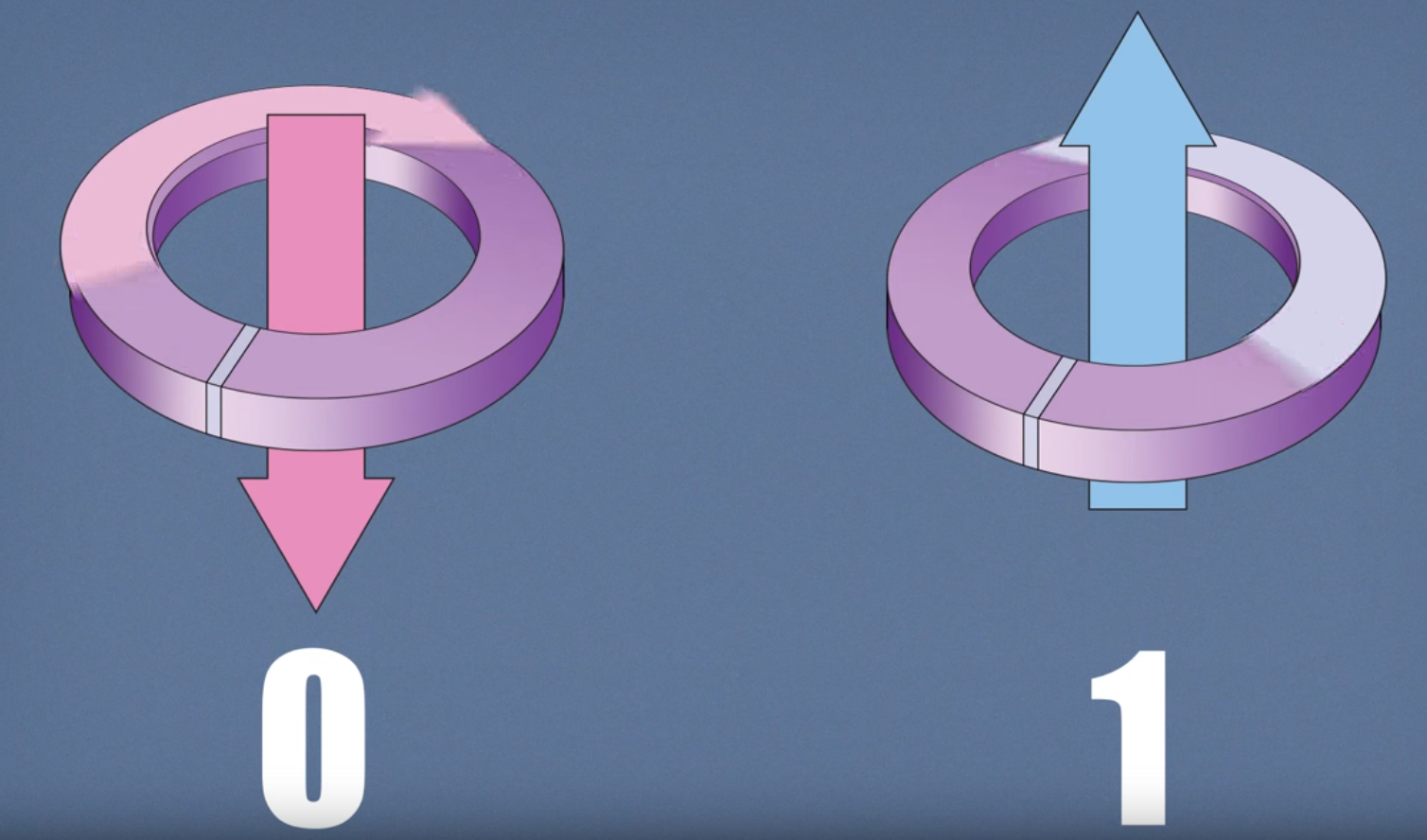
Fig. 6 A qubit’s state is implemented as a circulating current, shown clockwise for 0 and counterclockwise for 1, with a corresponding magnetic field.#
The physics of this process can be visualized with an energy diagram. At the start of the annealing process, the qubit is in a superposition state, which can be represented as a single valley with a single minimum energy. As the quantum annealing process runs, an energy barrier is raised which separates the single minimum energy into two valleys (that is, a double-well potential). For example, Figure 7 shows the energy diagram for the annealing process of a single qubit that results in two valleys of equal energy minima; thus the qubit has a 50/50 chance of being in either valley at the end of the anneal—that is, in the classical state of either 0 or 1.
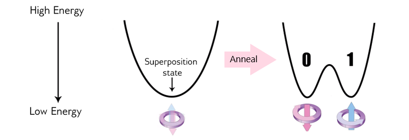
Fig. 7 Annealing process’s energy diagram shows raising the energy barrier for a single qubit, resulting in a 50/50 probability of ending in a classical state of 0 or 1.#
The probability of the qubit falling into the 0 or 1 state can be controlled by applying an external magnetic field to bias the qubit to end in one state over the other; the magnetic field is programmatically controlled via a qubit bias. For example, Figure 8 shows a magnetic field being applied to a single qubit as the energy barrier is raised; the magnetic field tilts the valleys in a preferred direction, increasing the probability of the qubit ending up in the valley with the lower energy minimum—here, the classical state of 1.
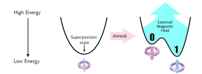
Fig. 8 Annealing process’s energy diagram shows an external magnetic field being applied to a single qubit, resulting in a higher probability of ending in a classical state of 1.#
However, the real power of quantum annealing is realized when you link qubits together so they can influence each other, accomplished via a device called a coupler. A coupler can correlate two qubits such that they tend to end up in the same classical state—both 0 or both 1—or in opposite states. The correlation between coupled qubits is controlled programmatically. Together, programmable qubit biases and coupler correlations are the means by which a problem is defined in the D-Wave quantum computer.
Furthermore, couplers use another phenomenon of quantum physics called entanglement. When two qubits are entangled, they can be thought of as a single object with four possible states. Figure 9 illustrates this idea, showing a potential with four states, each corresponding to a different combination of the two qubits: (0,0), (0,1), (1,1), and (1,0). The relative energy of each state depends on the biases of qubits and the couplers between them. During the anneal, the qubit states are potentially entangled in this landscape before finally settling into (1,1) at the end of the anneal.
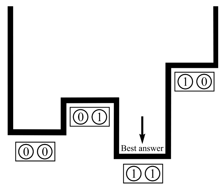
Fig. 9 Energy diagram showing the best answer.#
As stated, each qubit has a bias and qubits interact via the couplers. When formulating a problem, you choose values for the qubit biases and couplers. The qubit biases and couplers define an energy landscape, and the D-Wave quantum computer finds the minimum energy of that landscape: this is quantum annealing.
Systems get increasingly complex as qubits are added: two qubits have four possible states over which to define an energy landscape; three qubits have eight. Each additional qubit doubles the number of states over which you can define the energy landscape: the number of states goes up exponentially with the number of qubits.
In summary, the system starts with a set of qubits, each in a superposition state of 0 and 1. They are not yet coupled. When they undergo quantum annealing, the couplers and qubit biases are introduced and the qubits become entangled. At this point, the system is in an entangled state of many possible answers. By the end of the anneal, each qubit is in a classical state that represents the minimum energy state of the problem, or one very close to it. All of this happens in D-Wave quantum computers in a matter of microseconds.
Underlying Quantum Physics#
This section discusses some concepts essential to understanding the quantum physics that governs the D-Wave quantum annealing process.
The Hamiltonian and the Eigenspectrum#
A classical Hamiltonian is a mathematical description of some physical system in terms of its energies. You can input any particular state of the system, and the Hamiltonian returns the energy for that state. For most non-convex Hamiltonians, finding the minimum energy state is an NP-hard problem that classical computers cannot solve efficiently.
As an example of a classical system, consider an extremely simple system of a table and an apple. This system has two possible states: the apple on the table, and the apple on the floor. The Hamiltonian tells you the energies, from which you can discern that the state with the apple on the table has a higher energy than that when the apple is on the floor.
For a quantum system, a Hamiltonian is a function that maps certain states, called eigenstates, to energies. Only when the system is in an eigenstate of the Hamiltonian is its energy well defined and called the eigenenergy. When the system is in any other state, its energy is uncertain. The collection of eigenstates with defined eigenenergies make up the eigenspectrum.
For the D-Wave quantum computer, the Hamiltonian may be represented as
where \({\hat\sigma_{x,z}^{(i)}}\) are Pauli matrices operating on a qubit \(q_i\), and \(h_i\) and \(J_{i,j}\) are the qubit biases and coupling strengths.[1]
The Hamiltonian is the sum of two terms, the initial Hamiltonian and the final Hamiltonian:
Initial Hamiltonian (first term)—The lowest-energy state of the initial Hamiltonian is when all qubits are in a superposition state of 0 and 1. This term is also called the tunneling Hamiltonian.
Final Hamiltonian (second term)—The lowest-energy state of the final Hamiltonian is the answer to the problem that you are trying to solve. The final state is a classical state, and includes the qubit biases and the couplings between qubits. This term is also called the problem Hamiltonian.
In quantum annealing, the system begins in the lowest-energy eigenstate of the initial Hamiltonian. As it anneals, it introduces the problem Hamiltonian, which contains the qubit biases and couplers, and it reduces the influence of the initial Hamiltonian. At the end of the anneal, it is in an eigenstate of the problem Hamiltonian. Ideally, it has stayed in the minimum energy state throughout the quantum annealing process so that—by the end—it is in the minimum energy state of the problem Hamiltonian and therefore has an answer to the problem you want to solve. By the end of the anneal, each qubit is a classical object.
Annealing in Low-Energy States#
A plot of the eigenenergies versus time is a useful way to visualize the quantum annealing process. The lowest energy state during the anneal—the ground state—is typically shown at the bottom, and any higher excited states are above it; see Figure 10.
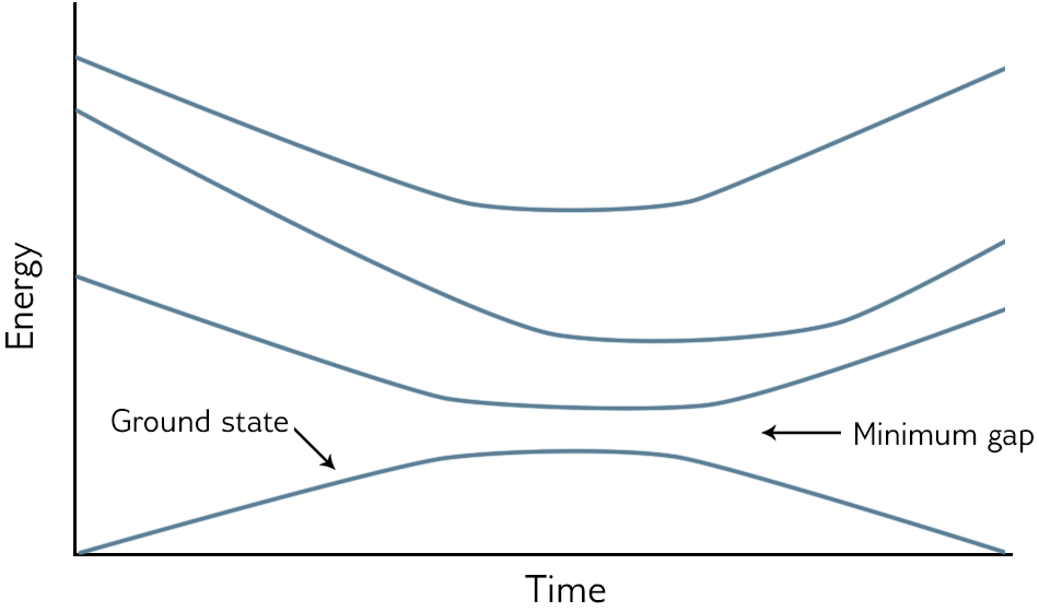
Fig. 10 Eigenspectrum, where the ground state is at the bottom and the higher excited states are above.#
As an anneal begins, the system starts in the lowest energy state, which is well separated from any other energy level. As the problem Hamiltonian is introduced, other energy levels may get closer to the ground state. The closer they get, the higher the probability that the system will jump from the lowest energy state into one of the excited states. There is a point during the anneal where the first excited state—that with the lowest energy apart from the ground state—approaches the ground state closely and then diverges away again. The minimum distance between the ground state and the first excited state throughout any point in the anneal is called the minimum gap.
Certain factors may cause the system to jump from the ground state into a higher energy state. One is thermal fluctuations that exist in any physical system. Another is running the annealing process too quickly. An annealing process that experiences no interference from outside energy sources and evolves the Hamiltonian slowly enough is called an adiabatic process, and this is where the name adiabatic quantum computing comes from. Because no real-world computation can run in perfect isolation, quantum annealing may be thought of as the real-world counterpart to adiabatic quantum computing, a theoretical ideal. In reality, for some problems, the probability of staying in the ground state can sometimes be small; however, the low-energy states that are returned are still very useful.
For every different problem that you specify, there is a different Hamiltonian and a different corresponding eigenspectrum. The most difficult problems, in terms of quantum annealing, are generally those with the smallest minimum gaps.
Evolution of Energy States#
Figure 11 shows the dependence of the \(A\) and \(B\) parameters in the Hamiltonian on s, the normalized anneal fraction, an abstract parameter ranging from 0 to 1. The \(A(s)\) curve is the tunneling energy and the \(B(s)\) curve is the problem Hamiltonian energy at \(s\). Both are expressed as energies in units of Joules as is standard for a Hamiltonian. A linear anneal sets \(s = t / t_f\), where \(t\) is time and \(t_f\) is the total time of the anneal. At \(t=0\), \(A(0) \gg B(0)\), which leads to the quantum ground state of the system where each spin is in a delocalized combination of its classical states. As the system is annealed, \(A\) decreases and \(B\) increases until \(t_f\), when the final state of the qubits represents a low-energy solution.
At the end of the anneal, the Hamiltonian contains the only \(B(s)\) term. It is a classical Hamiltonian where every possible classical bitstring (that is, list of qubit states that are either 0 or 1) corresponds to an eigenstate and the eigenenergy is the classical energy objective function you have input into the system.
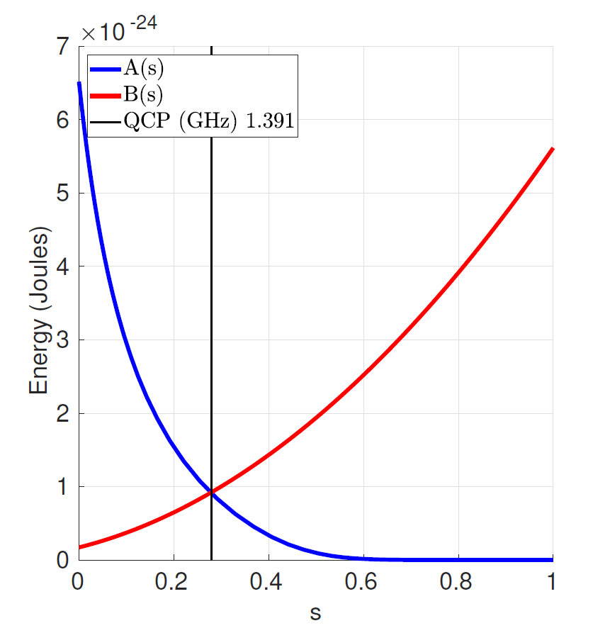
Fig. 11 Annealing functions \(A(s)\), \(B(s)\). Annealing begins at \(s=0\) with \(A(s) \gg B(s)\) and ends at \(s=1\) with \(A(s) \ll B(s)\). Data shown are representative of D-Wave 2X systems.#
Annealing Controls#
D-Wave continues to pursue a deeper understanding of the fine details of quantum annealing and devise better controls for it. The quantum computer includes features that give users programmable control over the annealing schedule, which enable a variety of searches through the energy landscape. These controls can improve both optimization and sampling performance for certain types of problems, and can help investigate what is happening partway through the annealing process.
For more information about the available annealing controls, see QPU Solver Datasheet.