Other Error Sources#
As well as the ICE effects discussed at length in the Error Sources for Problem Representation chapter, a number of other factors may affect system performance, including temperature, high-energy photon flux, readout fidelity, programming errors, and spin-bath polarization. This chapter looks at each of these in turn. For guidance on how to work around some of these factors to get improved performance, see the D-Wave Problem-Solving Handbook guide.
Temperature#
In a formal sense, temperature is defined for a system in thermodynamic equilibrium. In a practical sense, however, if the equilibrium time of a given subsystem is very short compared to the relaxation time between subsystems, then that subsystem may not be in thermal equilibrium with other subsystems capable of exchanging energy.
For example, the superconducting QPU and the block of metal attached to both it and a separate low-temperature thermometer have distinct temperatures. The thermometer measures the temperature of the dilution refrigerator’s mixing chamber; however, this may be a couple of millikelvin colder than the QPU. Furthermore, there is a distinction between the temperature of the quasiparticles in a superconducting wiring layer of the QPU and its phonons, and between the phonons of the wiring layer and those of the silicon substrate.
For timescales over which the annealing algorithm operates, the qubits are considered to be in equilibrium with a thermal bath at an effective temperature that can be measured, for example, by looking at the equilibrium distribution of single, uncoupled qubits when held in a fixed longitudinal and transverse field. (See Figure 81 and [Joh2011], Supplemental Information, section II.D page 8.)
Ensuring that a QPU operates at millikelvin-scale temperatures requires minimizing the amount of energy deposited on the QPU, as well as ensuring that energy is efficiently removed from it. Nevertheless, some heat is dissipated on the QPU during normal operation, particularly during the programming cycle. This can, depending on the frequency of programming, increase the effective temperature of the qubits and therefore affect solution quality.
Temperature effects vary from QPU to QPU, and depend on a number of manufacturing-related details. In practice, the effects can be quantified by performing the aforementioned equilibrium distribution tests when no programming is being performed and again when programming is done at maximum frequency, and then comparing the values.[1]
Note
Contact D‑Wave Customer Support to obtain the detailed properties of your system.
As a simple illustration of the effect of thermal equilibration, consider a single-qubit problem. As shown in Figure 84, you find that single qubits freeze out at an \(s\) value of roughly \(0.7\). At that point, \(B(s)\)—for the particular QPU shown—is approximately 7 GHz. Before this freezeout point, you can assume that the single qubits are in thermal equilibrium at some temperature \(T\) after which no further dynamics are present. At \(s = 0.7\), an applied \(h\) of \(1.0\) to the single qubit results in an energy difference between the up and down states of 7 GHz. The expected distribution for the spin up population is: \(P_{\uparrow} / 1-P_{\uparrow} = e^{-\delta E / k_b T}\).
Because \(\delta E = B(s) h\), you can sweep \(h\) over a small range and fit the result to a hyperbolic tangent and extract the resulting \(T\) of the QPU. Figure 104 shows the results of a measurement where you sweep the \(h\) values on all the qubits on a QPU, shift the curves to have the same centers, and then fit the averaged data to a hyperbolic tangent to extract the effective temperature of the qubits.
As a consequence, even when the temperature of the mixing chamber is constant, the effective temperature of the qubits may vary by a few millikelvin, depending on usage.
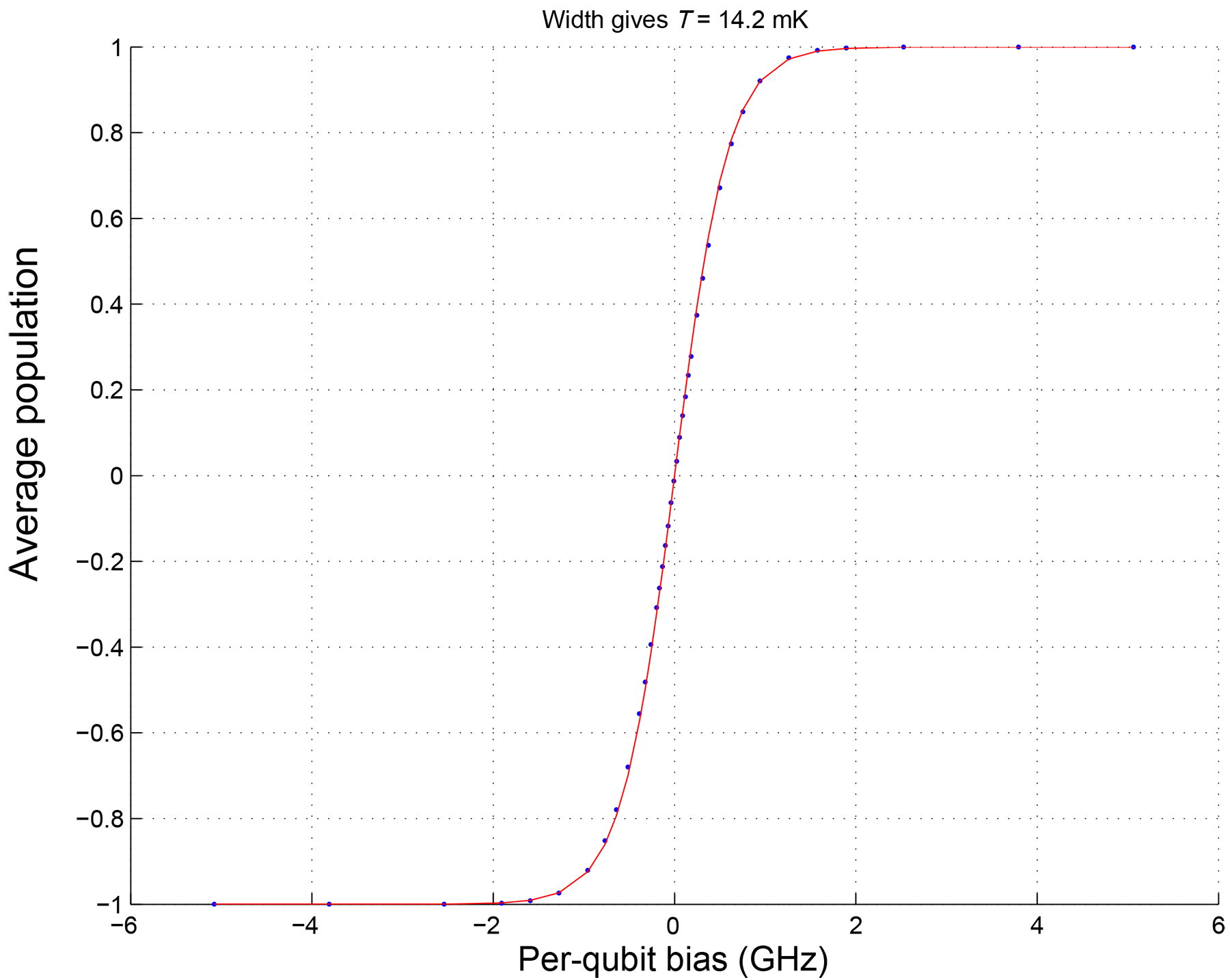
Fig. 104 Single qubit temperature extraction: Sampling the trivial 1-qubit problem, \(H = -h_i s_i\) on the QPU for qubit \(i\) (averaged over all qubits after centering each data set) for several values of \(h_i\) on the x-axis, results in the blue points shown in this plot. Fitting the data to a Boltzmann distribution gives the red curve and allows us to extract an effective temperature of \(14.2\) mK for this sample data. Conversion from \(h_i\) to energy bias is done by looking at the anneal schedule \(B(s)\) at the single qubit freezeout point in Figure 84.#
High-Energy Photon Flux#
The presence of relatively high-energy photons also plays a role. High-energy, in this context, means that photon energy and population exceed what would be expected at equilibrium at the measured effective qubit temperature.
These photons enter the QPU from higher-temperature stages through cryogenic filtering. When the annealing algorithm runs, they can cause transitions to much higher-energy problem states than would be expected given the equilibrium picture discussed in the previous section. Given a constant flux of high-energy photons, the probability of such a transition should increase the longer the annealing algorithm takes. This phenomenon may manifest as an appearance of solutions with energies much higher than the expected thermal distribution. This effect grows with longer anneal times.
Note
The anneal schedule feature discussed the Varying the Global Anneal Schedule section allows you to insert pauses at intermediate values of \(s\). Be aware that pausing at intermediate points in the quantum annealing process may increase the probability of transitions to higher energy states. As with the standard annealing schedule, the phenomenon may manifest as an appearance of solutions with energies much higher than the expected thermal distribution of energies and the effect grows with pause time.
Readout Fidelity#
Readout fidelity is not typically a significant factor in the D‑Wave quantum computer. Averaged over an ensemble of randomized bit strings, the typical readout fidelity of the system is greater than 99%. That is, one out of every 100 reads of a given problem may report a solution that is different from that found by the QPU by one or more bit flips.
For guidelines on how to use multiple reads to identify readout errors and make the best use of QPU time, see the D-Wave Problem-Solving Handbook guide.
Programming Errors#
A problem that uses all available qubits and couplers has a greater than 90% chance of being programmed without error. Occasionally, however, programming (or reset) issues occur during the programming cycle of the QPU, moving the problem implementation on the QPU far enough away from the intended problem that the solutions computed by the QPU do not overlap the low-energy subspace of the intended problem. If low-energy answers for a single problem are critical, submit the problem at least twice.
Note
Spin-reversal transforms reprogram the system and thereby offer another way to reduce the impact of these errors; for more information on this technique, see the D-Wave Problem-Solving Handbook guide.
Spin-Bath Polarization Effect#
One of the main sources of environmental noise affecting the qubit is magnetic fluctuations from an ensemble of spins local to the qubit wiring. This produces low-frequency flux noise that can cause the misspecification errors referred to in this document as “ICE 1.” In addition, the persistent current flowing in the qubit body during the quantum annealing algorithm produces a magnetic field that can partially align or polarize this ensemble of spins.
This partially polarized environment may bias the body of the qubit. This phenomenon may manifest, for example, in measurements of single qubit transition widths (the width of qubit population versus h bias). For very long anneal times, the polarized environment may add to the external h bias, producing a transition width that is narrower than the width expected from a thermal distribution. The partially polarized environment can also produce sample-to-sample correlations, biasing the QPU towards previously achieved spin configurations.
To reduce these sample-to-sample correlations, enable the reduce_intersample_correlation solver parameter. This setting adds optimal delay times before each anneal, giving the spin bath time to depolarize and thereby lose the effects from the previous read. It adds a delay that varies (approximately) between \(200\) microseconds and \(10\) milliseconds, increasing linearly with increasing length of the schedule:
where T is the total time of the anneal schedule.
Important
Enabling this parameter drastically increases problem run times. To avoid exceeding the maximum problem run time configured for your system, limit the number of reads when using this feature. For more information, see the Operation and Timing section.
The anneal schedule feature discussed in the Annealing Implementation and Controls chapter allows you to insert pauses at intermediate values of \(s\). Be aware that pausing at intermediate points in the quantum annealing process may increase the degree of polarization of the spin environment and thus the size of the bias back on the body of the qubit.