Error-Correction Features#
D‑Wave quantum computers provide some features to alleviate the effects of the errors described in previous chapters. Additionally, you can mitigate some effects through the techniques described in the D-Wave Problem-Solving Handbook guide.
Drift Correction#
Flux noise is described and its effects characterized in the Flux Noise of the Qubits and Characterizing the Effect of Flux Noise sections of the Error Sources for Problem Representation chapter.
By default, the D‑Wave system uses the following procedure to measure and
correct for the longest drifts once an hour. You can disable the application of
any correction by setting the flux_drift_compensation solver parameter to
False. If you do so, you should apply flux-bias offsets manually; see the
Calibration Refinement section.
The number of reads for a given measurement, \(N_\mathrm{reads}\), is set to 2000.
A measurement of the zero-problem, with all \(h_i = J_{i,j} = 0\) is performed, and the average spin computed for the \(i\)-th qubit according to \(\left<s_i\right> = \sum_j{s_i^{(j)}}/N_\mathrm{reads}\), where \(s_i^{(j)} \in \{+1,-1\}\) and the sum is performed over the \(N_\mathrm{reads}\) independent anneal-read cycles.
The flux offset drift of the \(i\)-th qubit is estimated as \(\delta\Phi_i = w_i\left<s_i\right>\), where \(w_i\) is the thermal transition width of qubit \(i\); defined below.
The measured \(\delta\Phi_i\) are corrected with an opposing on-QPU qubit flux–bias shift. The magnitude of the shift applied on any given iteration is capped to minimize problems due to (infrequent) large \(\delta\Phi_i\) measurement errors.
\(N_\mathrm{reads}\) is doubled, up to a maximum of 20,000.
The procedure repeats from step 2 at least 6 times. It repeats beyond 6 if the magnitude of any of the \(\delta\Phi_i\) after the last iteration is significantly larger than the expected variation due to \(1/f\) flux noise.
The thermal width, \(w_i\), of qubit \(i\) is determined during QPU calibration by measuring the isolated qubit (\(J_{i,j} = 0\) everywhere) average spin \(\left<s_i(\Phi_i^{(x)})\right>\) as a function of applied flux bias \(\Phi_i^{(x)}\) for each qubit, and fitting to the expression \(\tanh{\left[(\Phi_i^{(x)}-\Phi_i^{(0)})/w_i\right]}\), where \(\Phi_i^{(0)}\) and \(w_i\) are fit parameters.
For a typical \(w_i\) of order 100 \(\mu\Phi_0\), statistical error is measured at \(100~\mu\Phi_0/\sqrt{20000} \simeq 1~\mu\Phi_0\). This is much smaller than the root mean square (RMS) flux noise, which is on the order of 10 \(\mu\Phi_0\) for the relevant time scales.
Extended \(J\) Range#
Ising minimization problems that the D‑Wave system solves may require that the model representing a problem be minor-embedded on the working graph, a process that involves creating qubit chains to represent logical variables, as introduced in the minor-embedding chapter of the Getting Started with D-Wave Solvers guide. In an embedding, intra-chain qubit couplings must be strong compared to the input couplings between the chains.
Most discussions of chain strength involve the ratio of two absolute values:
Chain coupling strength—Magnitude of couplings between qubits in a chain
Problem scale—Maximum magnitude of couplings among qubits (physical or logical) in a problem
that is,
For example, if all of the chains have \(J\) values of \(-1\), and the rescaled[1] logical problem has \(J\) values of \(- \frac{1}{4}\) to \(+ \frac{1}{4}\), you say that the chain strength is \(4\). Likewise, if the chains have \(J\) values of \(-2\), and the rescaled logical problem has \(J\) values of \(- \frac{1}{2}\) to \(+ \frac{1}{2}\), again you say that the chain strength is \(4\).
Because the range of coupling strengths available is finite, chaining is typically accomplished by setting the coupling strength to the largest allowed negative value and scaling down the input couplings relative to that. Yet a reduced energy scale for the input couplings may make it harder for the QPU to find global optima for a problem.
To address this issue, some solvers support stronger chain couplings through an extended_j_range solver property. Because embedded problems typically have chain couplings that are at least twice as strong as the other couplings, and standard chain couplings are all negative, this feature effectively doubles the energy scale available for embedded problems; see Figure 105.
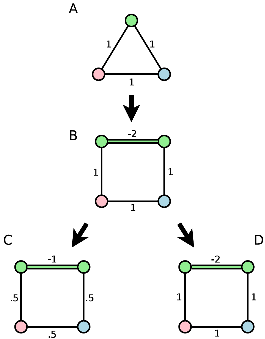
Fig. 105 Embedding an input that does not fit directly on a D‑Wave QPU. The original problem (A) has a green vertex that is replaced by a chain of two vertices connected with a ferromagnetic coupling (B). With the standard coupling range, the embedded problem must be scaled down for the QPU, which can lead to decreased performance (C). However, with an extended coupling range, no rescaling is necessary (D).#
Using the available larger negative values of \(J\) increases the dynamic \(J\) range. On embedded problems, which use strong chains of qubits to build the underlying graph, this increased range means that the problem couplings are less affected by ICE and other effects. However, strong negative couplings can bias a chain and therefore flux-bias offsets might be needed to recalibrate it to compensate for this effect; see the Calibration Refinement section for more information.
Calibration Refinement#
In an optimal QPU calibration, annealing unbiased qubits produces spin-state statistics that are equally split between spin-up and spin-down. When plotted against the \(h\) values, this even distribution results in a sigmoid curve that passes through the point of origin (0,0). However, non-idealities in QPU calibration and coupling to its environment result in some asymmetry. This asymmetry typically increases under strong coupling (such as when the extended_j_range is used for chains): a \(J\)-induced bias (an offset magnetic field that is potentially \(s\)-dependent).[2]. These effects shift the sigmoid curve of plotted \(h\) values from its ideal path, as shown in Figure 106.
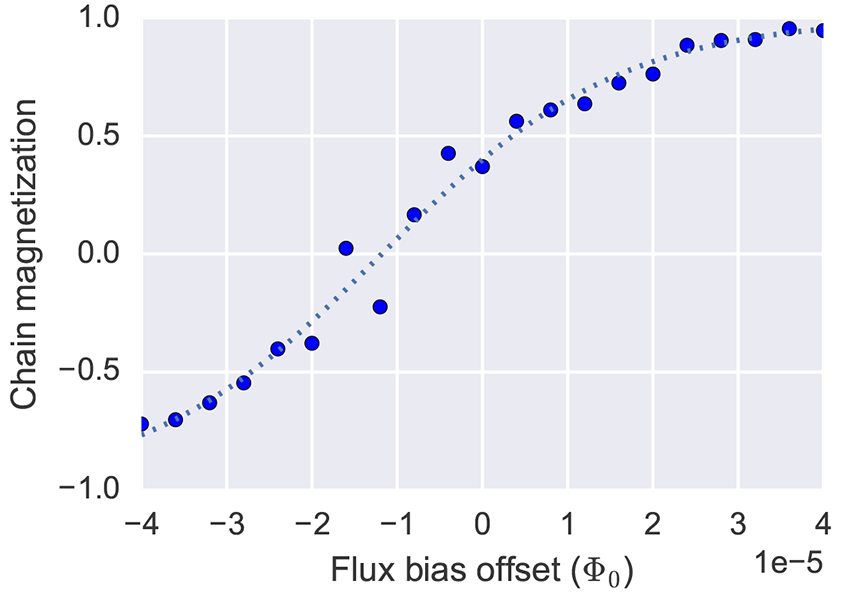
Fig. 106 Magnetization (mean spin value) of a six-qubit chain on an Advantage2™ QPU as a function of applied per-qubit flux-bias offset. A sigmoid function (\(\tanh()\), the dashed line) fit to the measurements intersects the horizontal grid line slightly above the zero.#
While the effect may be minor for many optimization problems, for others, such as material simulation, it may be significant. You can compensate by refining the calibration, applying per-qubit flux_biases to nudge the plotted \(h\) sigmoid to its ideal position.
Flux biases can be used to refine the standard calibration. [Che2023] describes (and links to code) techniques that tune the Hamiltonian to reduce the differences between the symmetric ideal and the asymmetric measurements on the QPU.
Note
The applied flux bias is constant in time (and \(s\)), but it appears in the Hamiltonian shown in equation (3) as a term \(I_p \phi_{\rm flux bias} \sigma_z\)—the applied energy grows as \(\sqrt{B(s)}\). An applied flux bias is different from an applied \(h\); do not use one to correct an error in the other.
Virtual Graphs#
Important
The virtual graph feature is deprecated due to improved calibration of
newer QPUs: Ocean software’s
VirtualGraphComposite class will be
removed in a future release. To calibrate chains for residual biases, follow
the instructions in [Che2023].
The D‑Wave virtual graph feature (see the
VirtualGraphComposite
class) simplifies the process of minor-embedding by enabling you to more easily
create, optimize, use, and reuse an embedding for a given working graph. When
you submit an embedding and specify a chain strength using these tools, they
automatically calibrate the qubits in a chain to compensate for the effects of
biases that may be introduced as a result of strong couplings. For more
information on virtual graphs, see
Virtual Graphs for High-Performance Embedded Topologies, D‑Wave White
Paper Series, no. 14-1020A, 2017. This and other white papers are available from
https://www.dwavesys.com/resources/publications.
Virtual graphs make use of Extended J Range and Calibration Refinement features. These controls allow chains to behave more like physical qubits on the working graph, thereby improving the performance of embedded sampling and optimization problems.
Note
Despite the similarity in name, the virtual graphs feature is unrelated to D‑Wave’s virtual full-yield chip (VFYC) solver.
Whether virtual graph features are available may vary by solver; check for the extended_j_range property to see if it is present and what the range is. (The j_range property is unchanged.) When using an extended \(J\) range, be aware that there are additional limits on the total coupling per qubit: the sum of the \(J\) values for each qubit must be in the range specified by the per_qubit_coupling_range solver property.
Flux-biases are set through the flux_biases parameter, which takes a list of doubles (floating-point numbers) of length equal to the number of working qubits. Flux-bias units are \(\Phi_0\); typical values needed are \(< 10^{-4} \ \Phi_0\). Maximum allowed values are typically \(> 10^{-2} \ \Phi_0\). The minimum step size is smaller than the typical levels of intrinsic \(1/f\) noise; see the Characterizing the Effect of Flux Noise section.
Note
By default, the D‑Wave system automatically compensates for flux drift as described in the Characterizing the Effect of Flux Noise section. If you choose to disable this behavior, you should apply flux-bias offsets manually through the flux_biases parameter.
Be aware of the following points when using virtual graph features:
Autoscaling is not supported with flux-bias offsets. When you use this feature, autoscaling is automatically disabled by default, unlike in the usual system behavior.
The \(J\) value of every coupler must fall within the range advertised by the extended_j_range property.
The sum of all the \(J\) values of the couplers connected to a qubit must fall within the per_qubit_coupling_range property. For example, if this property is
[-9.0 6.0], the following \(J\) values for a six-coupler qubit are permissible:\[1, 1, 1, 1, 1, 1,\]where the sum is \(6\), and also
\[1, 1, 1, -2, -2, -2,\]where the sum is \(-3\). However, the following values, when summed, exceed the range and therefore are impermissible:
\[-2, -2, -2, -2, -2, -2.\]While the extended \(J\) range in principle allows you to create almost arbitrarily long chains without breakage, the maximum chain length where embedded problems work well is expected to be in the range of 5 to 7 qubits.
When embedding logical qubits using the extended \(J\) range, limit the degree, \(D\), of each node in the logical qubit tree to
\begin{equation} \begin{array}{rcl} D &=& {\rm floor} \bigg[ \frac{\min(per\_qubit\_coupling\_range)}{\min(extended\_j\_range) - \min(j\_range)} \\ & & -\frac{num\_couplers\_per\_qubit \times \min(j\_range)} {\min(extended\_j\_range) - \min(j\_range)} \bigg] \end{array} \end{equation}where \(num\_couplers\_per\_qubit = 5\) for the Advantage™ QPU; see the QPU Architecture section of the Getting Started with D-Wave Solvers guide.