Appendix: Benefits of Postprocessing

Postprocessing optimization and sampling algorithms provide local improvements with minimal overhead to solutions obtained from the quantum processing unit (QPU).

Server-side postprocessing for Advantage systems is limited to computing the energies of returned samples[1] but Ocean software provides additional client-side postprocessing tools (see, for example, the Postprocessing with a Greedy Solver documentation).

[1]

Earlier D-Wave systems, such as the D-Wave 2000Q system, optionally provided additional postprocessing server-side.

This appendix provides an overview of some postprocessing methods for your consideration and presents the results of a number of tests conducted by D-Wave on the postprocessor of one of D-Wave’s previous quantum computers, the D-Wave 2000Q or DW2X systems.

Optimization and Sampling Postprocessing

For optimization problems, the goal is to find the state vector with the lowest energy. For sampling problems, the goal is to produce samples from a specific probability distribution. In both cases, a logical graph structure is defined and embedded into the QPU’s topology. Postprocessing methods are applied to solutions defined on this logical graph structure.

Optimization Postprocessing

The goal of optimization postprocessing is to obtain a set of samples with lowest energy on a graph \(G\). For simplicity of discussion, assume that \(G\) is a logical graph. Pseudocode for optimization postprocessing is shown below. The postprocessing method works by performing local updates to the state vector \(S\) based on low treewidth graphs. Specifically, the DecomposeGraph function uses a set of algorithms based on the minimum-degree [Mar1957] heuristic to decompose graph \(G\) into several low treewidth subgraphs that cover the nodes and edges of \(G\). The SolveSubgraph function is then used to update the solution on each subgraph to obtain a locally optimal solution \(s'\). SolveSubgraph is an exact solver for low treewidth graphs based on belief propagation on junction trees [Jen1990].

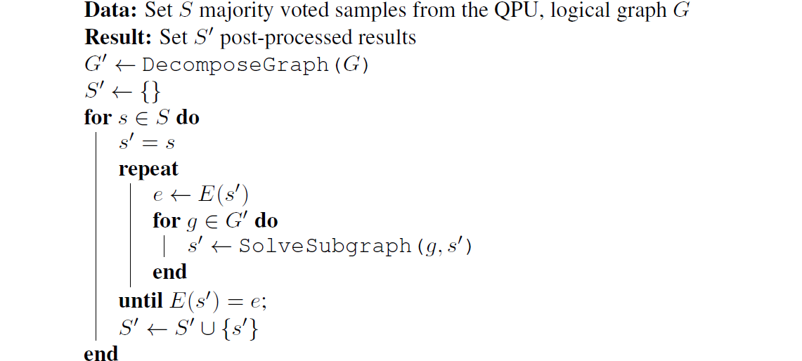
Fig. 110 Optimization postprocessing algorithm.

Sampling Postprocessing

In sampling mode, the goal of postprocessing is to obtain a set of samples that correspond to a target Boltzmann distribution with inverse temperature \(\beta\) defined on the logical graph \(G\). The pseudocode for sampling postprocessing is shown below. As with optimization postprocessing, the graph \(G\) is decomposed into low treewidth subgraphs \(G'\) that cover \(G\). On each subgraph, the state variables \(S\) obtained from the QPU are then updated using the SampleSubgraph function to match the exact Boltzmann distribution conditioned on the states of the variables outside the subgraph. Such algorithms should enable users to set the number of subgraph update iterations \(n\) and the choice of \(\beta\). Heuristically, this inverse temperature depends on model parameters in the Hamiltonian. As a general rule, \(\beta\) should be set to a value close to an inverse temperature corresponding to raw QPU samples. Some variation from a classical Boltzmann distribution is expected in postprocessed samples. See Sampling Tests and Results for discussion.

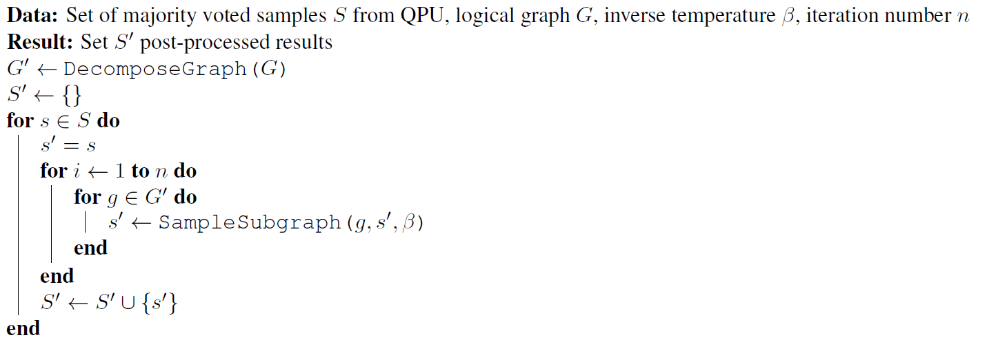
Fig. 111 Sampling postprocessing algorithm.

Optimization Tests and Results

This section describes a set of tests and results that examine the quality of results returned by the optimization postprocessor on one of D-Wave’s previous quantum computers, the D-Wave 2000Q system. The goal is to describe the difference between postprocessed solutions from those obtained solely via the QPU.

Postprocessing for optimization is evaluated by generating 10 random problems on a D-Wave QPU, each with \(J\) values drawn uniformly at random from \(\{1, -1\}\). Each problem is evaluated based on a set of scaling factors. Problems are scaled to exaggerate the negative effects of analog noise on solution quality, so the optimization postprocessor can demonstrate that it can recover a high-quality solution from the QPU solution. Specifically, with small scaling factors, it is difficult to faithfully represent problems in the QPU because of the exaggeration of analog noise. This noise causes the solver to return lower-quality solutions, and provides a nice mechanism to evaluate the optimization postprocessor.

For each problem and scaling factor, 1000 samples were drawn with postprocessing on and off. As seen in Figure 112 and Figure 113, postprocessing for optimization can improve solutions significantly. Furthermore, the worse the non-postprocessed solutions are, the more postprocessing helps.

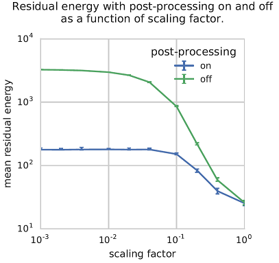
Fig. 112 Line plot of mean residual energies (mean energies above ground-state energy) returned by the D-Wave system with and without optimization postprocessing. Observe that optimization postprocessing does no harm, and helps more when scaling factors are smaller and the non-postprocessed samples not as good. Error bars indicate 95% confidence intervals over input Hamiltonians.

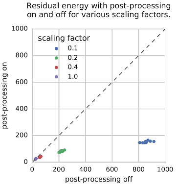
Fig. 113 Scatter plot of mean residual energies (mean energies above ground-state energy) returned by the D-Wave system with and without optimization postprocessing, with each point representing an input Hamiltonian. Observe that optimization postprocessing does no harm, and helps more when scaling factors are smaller and the non-postprocessed samples not as good.

Sampling Tests and Results

This section describes tests conducted to examine the quality of results returned by the sampling postprocessor on one of D-Wave’s previous quantum computers, the D-Wave 2000Q system. The goal is to describe the difference between postprocessed samples from those obtained solely via the QPU. Postprocessing is considered here at two different temperatures: an ultra-cold temperature, and a measured local temperature [Ray2016].

The results show that the energy improves for cold temperature, but at the cost of diversity. For the local temperature, diversity of postprocessed samples improves without compromising the energy distribution. Measures such as false-positive rate and backbone, defined below, complement the typical energy/entropy statistics. The results show that the backbone and false-positive rates are improved by low-temperature postprocessing. Together, these studies provide a glimpse into the behavior of QPU and postprocessed samples.

Methodology

The study considers a particular problem class: Not-All-Equal-3SAT (NAE3SAT), with 30 logical variables and a clause-to-variable ratio of 1.8. Each clause is a logical constraint on three variables, and the energy of a sample is linear in the number of clause violations.[2] This class was chosen because a variety of meaningful metrics can be used to analyze the raw QPU samples and the postprocessed results [Dou2015]. The embedding of this problem was chosen using the standard routine [Cai2014], and chain strength for the embedding was chosen by a heuristic rule that gave close-to-optimal results in terms of the fraction of ground states seen without postprocessing.

Sample quality is evaluated with respect to a target Boltzmann distribution using two values of \(\beta\): an ultra-cold temperature corresponding to \(\beta=10\) and a local estimate corresponding to \(\beta=2.0\). The cold temperature was chosen to be (for practical purposes) indistinguishable from the limiting case \(\beta\rightarrow \infty\). In this limited postprocessing, samples can only decrease in energy. This is a useful limit when the objective is to obtain ground-state, or low-energy, samples. In the examples presented, a significant fraction of samples are ground states both in the raw QPU sample set and in the postprocessed sample set. The local temperature is chosen so that before and after postprocessing, the sample-set mean energy is approximately unchanged. The local temperature can be estimated accurately by an independent procedure that probes the average energy change as a function of \(\beta\) [Ray2016]. Postprocessing at this local temperature should produce more diverse samples (higher entropy distributions) without increasing the average energy. This should be observed in the sampling metrics.

Figure 114 through Figure 118 show sample quality before and after postprocessing with \(n=10\), for various sampling metrics. Each pair of plots shows results from postprocessing at low temperature \(\beta=10\) (left) and local temperature \(\beta=2\) (right). Each panel shows results from 100 random NAE3SAT instances generated on 30 variables with clause-to-variable ratio 1.8. For each input, 1000 samples were collected from 10 different spin-reversal transforms for a total of 10,000 samples. The default annealing time of \(20 \ \mu s\) was used for all samples, and the postprocessor was applied with \(n=10\) steps. QPU samples have undergone embedding and chain-correction, and the following analysis is performed entirely in the logical space. Depending on the test being performed, sometimes only a subset of the samples were used. For example, it is convenient to define some metrics with respect to ground states only, or randomly select pairs of solutions to examine. Standard errors, and estimator bias (where relevant), are evaluated with the jackknife method [Efr1982].

Mean Energy

Figure 114 demonstrates the mean energy for solutions to the test problems compared before and after postprocessing. The mean energy is the expectation of the sample set energies; this estimator is unbiased and of small variance.

If you postprocess at low temperature, you hope to transform excited states into low-energy ones, so that you aim for a decrease in mean energy under postprocessing. In the cold case, shown on the left, the mean energy decreases dramatically after postprocessing, which is suggestive of successful postprocessing.

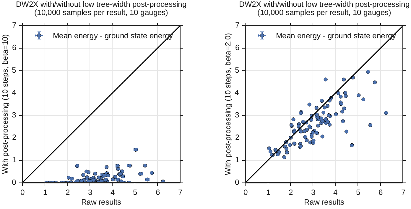
Fig. 114 Mean energy comparison of solutions to 100 NAE3SAT problems before and after postprocessing. Postprocessing is performed at \(\beta=10\) (left) and \(\beta=2\) (right). Postprocessing at \(\beta=10\) significantly reduces the energy of samples, whereas postprocessing at \(\beta=2\) does not. Standard errors are shown for each estimate, but these are in most cases small compared to the marker size.

If you postprocess at some other temperature, your aim is to approach the mean energy of the Boltzmann distribution at \(\beta\). The local temperature here is chosen so that to a first approximation energy should be unchanged under postprocessing. However, a single value of \(\beta\) is chosen for all NAE3SAT problems, so some upward or downward fluctuation in mean energy is expected in any given problem. Figure 114 (right) shows that, despite some fluctuations between problem instances, the mean energies before and after are, in the typical case, strongly correlated. This suggests only that the approximation to \(\beta\) local was appropriate for this class.

Entropy

Entropy is a measure of the size of the solution space. The aim of postprocessing at low temperature is to approach the ground-state entropy (a uniform distribution over ground states); in this process, the sample diversity is typically reduced. Successful postprocessing at the local \(\beta\) — chosen so that energy is approximately constant — leads to an increase in entropy. The Boltzmann distribution is the maximum entropy distribution for a given mean energy; therefore, if mean energy is unchanged, expect to see the largest value for entropy in the Boltzmann distribution.

The entropy for a distribution \(P(x)\) is defined as \(-\sum_x P(x)\log P(x)\), and can be estimated using samples drawn from \(P\). The Grassberger estimator [Gra2008] was used to measure the entropy from the sample sets. Figure 115 shows the relative entropy of the samples before and after postprocessing. At the cold temperature, the entropy decreases significantly, likely due to many of the excited states returned by the QPU being transformed into ground states. This also follows from the mean energy plot in Figure 114. At local \(\beta\), the entropy increases as one would expect. Low treewidth postprocessing allows the samples to diversify toward the maximum entropy distribution. This later choice of \(\beta\) allows a fair comparison of the two distributions since mean energy is controlled for; otherwise, entropy can always be improved by raising the mean energy of the distribution.

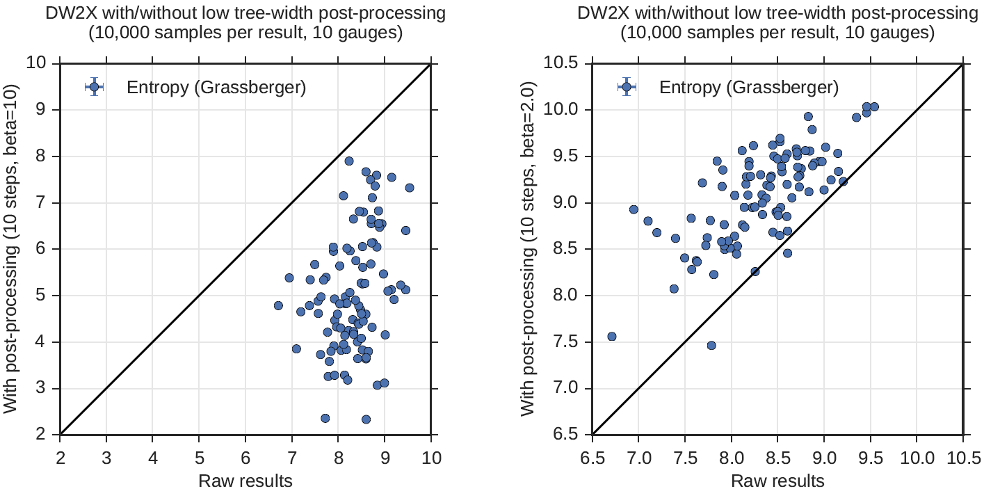
Fig. 115 Entropy comparison of solutions to 100 NAE3SAT problems before and after postprocessing. Postprocessing is performed at \(\beta=10\) (left) and \(\beta=2\) (right). Postprocessing at \(\beta=10\) reduces the entropy whereas postprocessing at \(\beta=2\) increases it.

KL Divergence

The Kullback–Leibler (KL) divergence is defined as \(\beta\) Energy \(-\) Entropy \(+ \log(Z(\beta))\), where \(Z(\beta)\) is a constant called the partition function. It is an important measure of distributional distance and is bounded below by zero. Postprocessing typically has a trade-off between mean energy and entropy. Distributions of high diversity (e.g., random samples) typically have higher energy; KL divergence is able to capture the trade-off between decreasing mean energy and increasing entropy. For any \(\beta\), as a distribution approaches the Boltzmann distribution, its KL divergence decreases toward zero. Postprocessing as undertaken here is guaranteed to decrease KL divergence. The more successful the postprocessing is, the larger the decrease, and the closer the postprocessed distribution is to zero.

To demonstrate the effectiveness of postprocessing, you need not know the constant \(\log(Z)\); present instead \(KLD' = (KLD-log(Z))/\beta\). Figure 116 shows a significant and consistent decrease in KL divergence for all cases. In the cold case, the improvement in KL divergence is largely due to decreases in the mean energy. For the local temperature postprocessing, the decrease is a result of increased sample diversity.

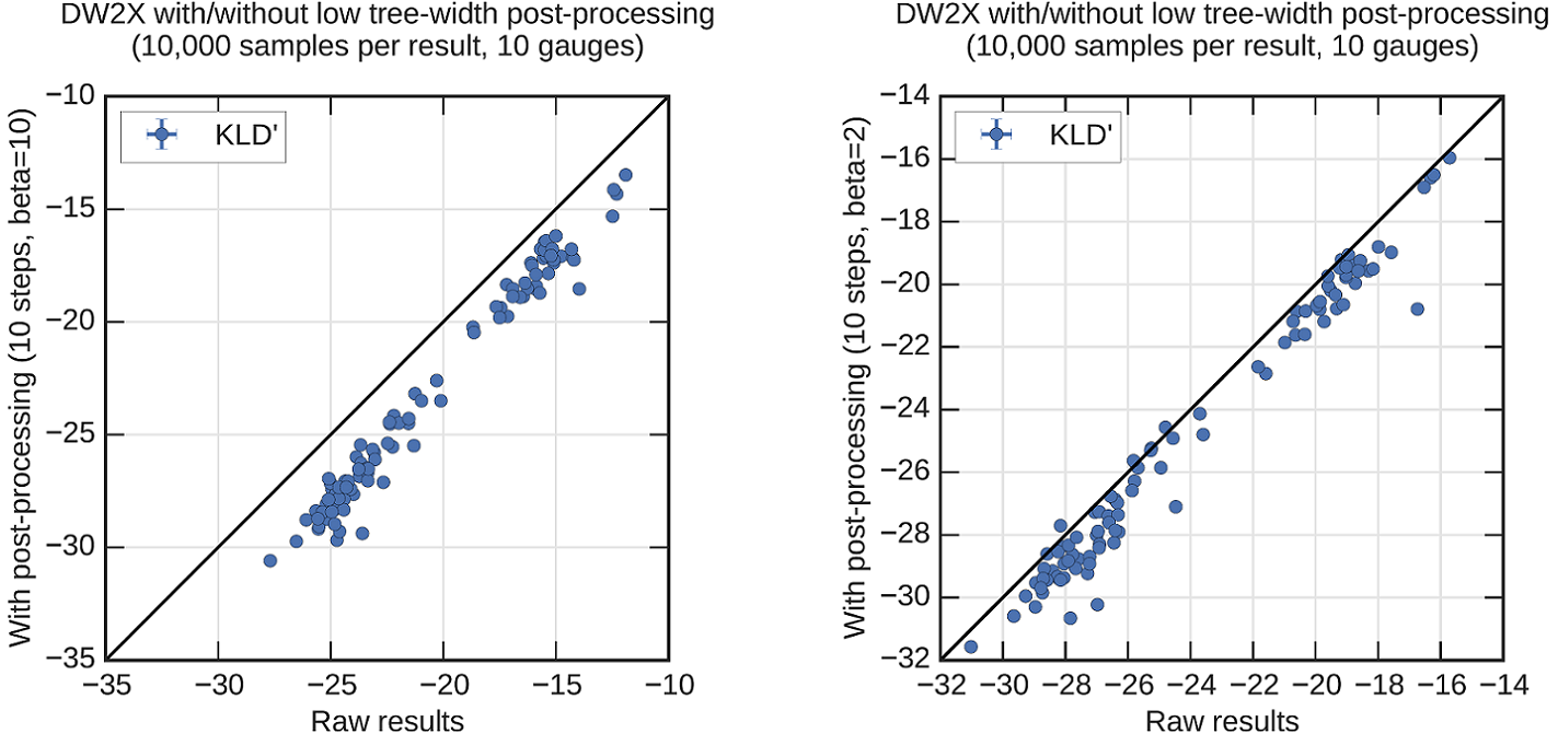
Fig. 116 \(KLD'\) comparison of solutions to 100 NAE3SAT problems before and after postprocessing. Postprocessing is performed at \(\beta=10\) (left) and \(\beta=2\) (right). In both cases, postprocessing improves the KL divergence, though the improvement is more significant at \(\beta=10\).

Backbone

If you restrict attention to the subset of samples that are ground states, you can define the backbone as the set of all variables that are perfectly correlated. Since the problem is symmetric, it is most interesting to consider edge states rather than spin states; to consider the number of correlations among variable pairs that are perfect (either perfect alignment or antialignment). The measure is interesting only for problems with ground-state degeneracy, such as NAE3SAT.

Define the backbone over edge variables for a distribution \(P\) as

\begin{equation} b = \frac{1}{\left|E\right|} \sum_{(i, \ j) \in E}^{E} I\left(|\langle x_i x_j\rangle_{GS}| \equiv 1\right), \end{equation}

where \(E\) is the set of edges in the problem, \(x_i\) is the spin state of variable \(i\), and angled brackets indicate an average with respect to the distribution over ground states (for the energy function of interest). \(I()\) is an indicator function, evaluating to 1 when the argument is true. For a distribution that has nonzero probability to see all ground states, the backbone is equal to that of the Boltzmann distribution[3]. If the distribution covers only a subset of ground states, the backbone is larger than the Boltzmann distribution. In the special case that only a single ground state is observed, the maximum value (1) is obtained.

Estimate the backbone from a finite set of samples drawn from \(P\) by replacing \(\langle x_i x_j\rangle\) with an empirical estimate[4]. This estimator is sensitive to not only whether the distribution supports a given ground state, but also how frequently the ground state is sampled. For a finite number of samples, the backbone is minimized by a distribution that is well spread across the ground state[5]. Consider the special case of a sampler that mostly sees a single ground state. If you only draw a few samples, the backbone is estimated as 1, even if by drawing many samples you would see the correct result. By contrast, if many diverse samples are drawn, a much smaller value is found. The Boltzmann distribution is uniform on the ground states and has a small backbone. Effective postprocessing reduces the estimate of the backbone as sample diversity increases and the Boltzmann distribution is approached.

Figure 117 shows the expected backbone when subsampling only two samples from the distribution. After postprocessing is applied with the cold temperature, the average backbone estimate produced by the sample improves overall. The trend is similar but less pronounced at the local temperature.

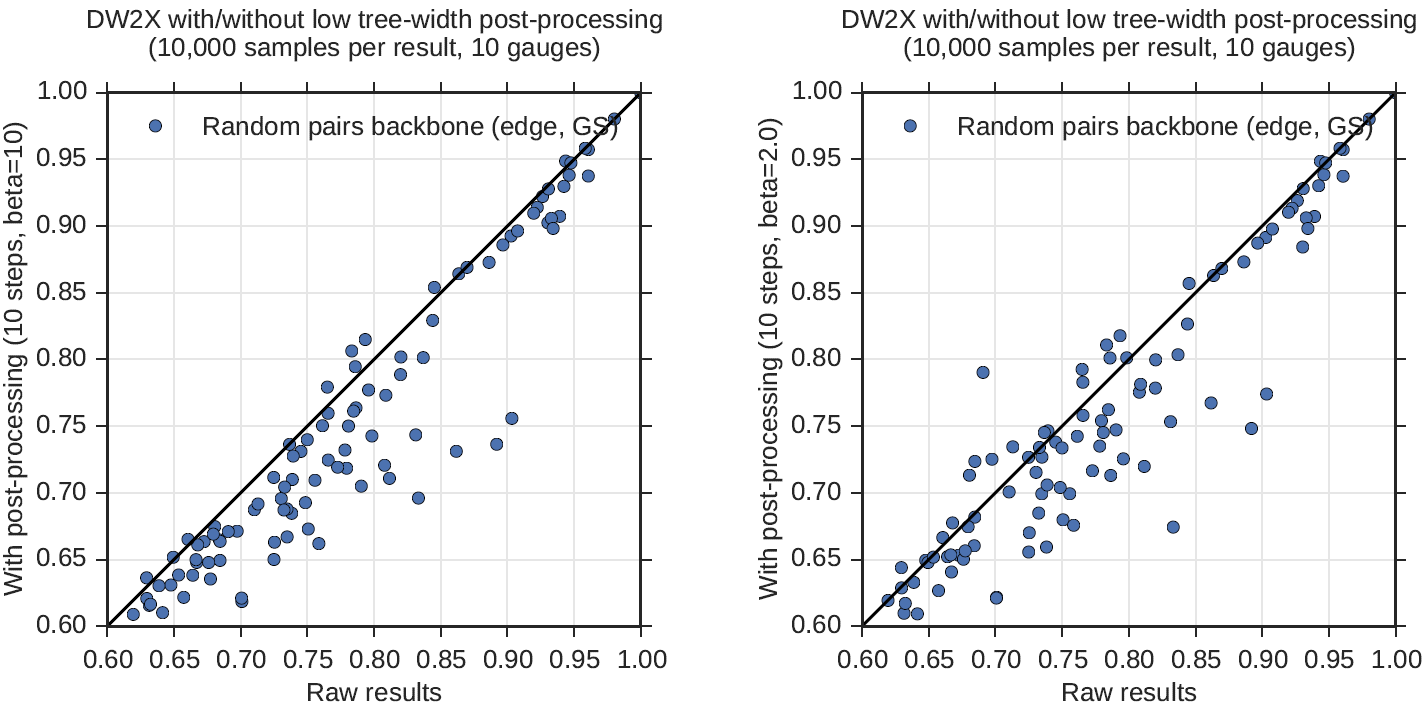
Fig. 117 Backbone comparison of solutions to 100 NAE3SAT problems before and after postprocessing. Postprocessing is performed at \(\beta=10\) (left) and \(\beta=2\) (right). In both cases, postprocessing improves the average backbone estimate overall, though the improvement is more significant at \(\beta=10\).

False-Positive Rate

One application of sampling is to create SAT filters [Dou2015]. A brief abstract description: the filter is defined by a set of samples, \(\mathcal{S}=\{x\}\), which are ground-state solutions to a satisfiable NAE3SAT problem instance. A test \(T\) of this filter is defined by a random triplet of indices, \(i_1,i_2,i_3\), and negations, \(n_1,n_2,n_3\). Indices are sampled uniformly from 1 to \(N\) (\(N=30\), the number of logical variables) without repetition; negations, from \(\pm 1\). The test yields either a false positive (1) if every sample in the set passes the test

$$\wedge_{x \in \mathcal{S}} I\left(\left|\sum_{l=1}^3 n_l x_{i_l}\right| \equiv 1\right)$$

or zero otherwise. The false-positive rate (FPR) for a given filter is an average over tests; the FPR for a distribution is an average over tests and sample sets of a given size.

Including a diverse set of samples (ground states) in the filter yields a lower FPR, for much the same reason as it reduces the backbone. This reduction in the FPR relates directly to filter effectiveness in application. Thus, postprocessing can be deemed successful if the set of ground states produced are diversified—yielding lower FPRs.

Figure 118 demonstrates the performance of filters. The FPR is determined by a double average over tests and sample sets. Filters were constructed from 1000 random sample pairs drawn without replacement from the larger sample set; to each was applied 1000 random tests. Postprocessing improves the FPR in the majority of cases, though the signal is not very strong. Trends in this metric are consistent with the backbone result, as would be expected because the backbone can be considered to place a limit on the FPR.

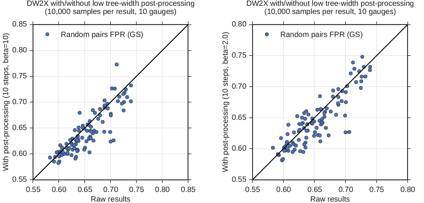
Fig. 118 Relative FPR comparison of solutions to 100 NAE3SAT problems before and after postprocessing. Postprocessing is performed at at \(\beta = 10\) (left) and \(\beta = 2\) (right). In both cases, postprocessing improves FPR overall, though the improvement is more significant at \(\beta = 10\).

[2]

The actual energy penalty for a clause violation is model dependent since the Hamiltonian is scaled to meet the QPU constraint on coupling strength.

[3]

All Boltzmann distributions see the ground states uniformly, though the probability to see a ground state is not uniform and increases with \(\beta\).

[4]

This finite set is drawn from the empirical set restricting to ground states and without replacement. This ensures that the estimate is independent from the fraction of samples that are ground states, which may vary between distributions.

[5]

A uniform distribution is expected to be close to optimal for many Hamiltonians, though it is not optimal in general.